Master’s Thesis in Informatics, Spring 2021
Artificial Intelligence Group
Department of Computer Science
Faculty of Information Technology and Electrical Engineering

Blank page
Abstract
Modern eye-tracking technology allows for the non-invasive evaluation of cognitive performance. Many systems for detecting cognition use features tailor-made to the given context and have limited use in other settings. There have been efforts to create generalized features from other data sources, but previous work has not addressed this for gaze data. In this study, we engineer a multitude of features and evaluate their generalizability across contexts. We utilize three datasets from different contexts and a machine learning platform to perform generalizability experiments. Our work presents several generalizable features and a novel architecture that can aid in engineering more such features from gaze data and other domains.
Oppsummering
Moderne blikksporingsteknologi gjør det mulig med mindre sjenerende måling av kognitive ytelse. Kognisjonsevalueringssystemer bruker i dag skreddersydde egenskaper (features) til den gitte konteksten og har begrenset brukbarhet i andre sammenhenger. Tidligere har det vært forsøkt å lage generaliserbare egenskaper fra andre datakilder, men dette er ikke gjort for blikkdata. I dette studiet utvikler vi flere forskjellige egenskaper og evaluerer generaliserbarheten deres på tvers av kontekster. Vi utnytter tre datasett fra forskjellige kontekster og en maskinlæringsplattform for å utføre generaliserbarhetseksperimenter. Vårt arbeid presenterer flere generaliserbare egenskaper og en arkitektur som kan bistå i utviklingen av flere slike egenskaper fra blikkdata og andre datakilder.
Acknowledgment
We extend our deepest gratitude to our advisors Kshitij Sharma and Michalis Giannakos. Their assistance has been thought-provoking, engaging, and critical to our success. Further, we would like to thank Jennifer Olsen for providing the Fractions dataset. Pål and Johannes have made life in the office a true joy. Lastly, we would like to thank our families and Madeleine Loraas for their support and proofreading.
1. Introduction
1.1. Motivation
Modern user-adaptive systems rely on understanding the current cognitive capabilities of users [1, 2, 3]. However, many such systems rely primarily on tailor-made solutions to detect such capabilities [4, 5, 6]. By moving towards generalizable solutions for detecting cognitive performance, we can decrease our reliance on the time-consuming development of such detection systems.
Cognition describes the different workings of our mental capacities. Weintraub et al. [7] identified executive function, episodic memory, language, processing speed, working memory as the most critical cognition subdomains for health, success in school and work, and independence in daily functioning. The National Institutes of Health (NIH) Toolbox Cognition Batteries is a well-established set of tests of cognition [7]. While the tests in the NIH Toolbox are thorough and well tested, they are also quite involved and time-consuming. As such, an alternative to the Toolbox is needed for the evaluation of cognitive performance. Cognitive workload, measured and assessed using eye-tracking technology, could serve as an alternative [8, 9].
Cognitive workload describes the level of mental resources that one person requires to perform a task and naturally falls within the purview of cognitive performance. Cognitive load theory, first proposed by John Sweller, establishes the three domains of cognitive load as intrinsic, extraneous, and germane. Intrinsic is concerned with the complexities in the information being learned. Extraneous cognitive load is the load that stems from the presentation of the instructional material. Lastly, germane cognitive load is concerned with the learner’s personal characteristics and the amount of attention that is being applied when learning [10, 11, 12]. Cognitive workload has also been shown to influence one’s eye movements [9, 13, 14].
Our project will include data gathered from studies handling many different cognitive tasks. We will argue that each task has some measure, such as a score, that correlates to the cognitive performance for that task.
1.1.1. Eye-Tracking
Eye-tracking is the process of tracking and recording the position of a subject’s gaze while interacting with digital devices. The gaze point for each of the eyes of a subject is recorded over time. Eye-tracking can be used as input control for interacting with systems [15], or to record user behavior when interacting with digital and physical systems [16, 17]. As the equipment involved has become cheaper and eye-tracking with web cameras has improved [18], eye-tracking has emerged as a promising non-invasive way to evaluate many facets of interactions with digital systems. These include collaborative work in MOOC learners [19], collaboration when interacting with Intelligent Tutoring Systems [20, 21], and detecting task-demand [9, 14].
1.1.2. Generalizability
Universality and generalism of research are important concepts, and their role in information systems research is an ongoing debate [22, 23]. Davison et al. point out that one must be explicitly aware of the context of one’s research and avoid unjustified generalization [22]. Cheng et al. agree that a close look at the context of a study is critical. However, they underline that generalizability is the ultimate goal of research, and well-reasoned generalizability should be pursued [23]. Our work is acutely aware of the context of each of the datasets we use, and we will aim to engineer features that are generalizable to other contexts. We will evaluate the degree of generalizability of our experiments through analysis.
While generalizability is a goal of machine learning research, there is little focus on feature generalizability in the literature. By feature generalizability, we mean the extent to which extracted features can predict the same variable, in our case cognitive performance, in different contexts. Inspired by the methods of Sharma et al. [24], we aim to engineer features that exhibit feature generalizability. The usefulness of understanding the rationale behind features and how they might differ when predicting the same classification target on different types of data has been studied by Rogers et al. in the context of text mining [25]. Feature generalizability has also been considered a central goal in feature selection within music information retrieval [26]. It has also been shown to be important in predicting students' affect during learning [27].
Sharma et al. engineered generalizable features from physiological data and facial expressions. They present the results from four independent studies and perform cross-training and testing with combinations of these datasets to explore the generalizability of their features across contexts. To evaluate the generalizability of their experiments, they proposed a "feature generalizability index" metric [24].
1.2. Research Questions
We will follow the methodology of Sharma et al. to develop generalizable features from gaze data [24]. In the process, we will also develop and present a machine learning platform to effectively run experiments to investigate generalizability and produce features from gaze data.
Our research questions are as follows:
-
RQ 1 What are the most generalizable features for predicting cognitive performance using gaze data?
-
RQ 2 What are the most context-specific features for predicting cognitive performance using gaze data?
When finding the most generalizable features, we will necessarily discover features that exhibit a high degree of context-specificity.
The thesis will tackle the research questions through the following research objectives:
-
RO 1 Design and develop a platform that allows for generalizability experiments.
-
RO 2 Collect a wide range of eye-tracking datasets from cognitive tasks in different contexts.
-
RO 3 Perform experiments on the developed platform and the selected datasets to evaluate the generalizability and context-specificity of a range of features.
-
RO 4 Create a library of generalizable and context-sensitive gaze features that account for users’ cognitive performance.
1.3. Terminology
In this section, we will introduce the reader to a few key terms from the eye-tracking field.
The term fixation refers to when the eye holds steady on an object or a position. Fixations usually reflect attention to a stimulus [9]. When discussing fixations, we will often refer to the fixation duration, which is the amount between the start of the fixation and the end of the fixation.
Saccades are small rapid eye movements that occur between two fixations. Cognitive information is not processed during saccadic eye movements. However, studies have shown that they still can provide information about viewing behavior and indicate changes in cognition [9, 28]. We will primarily refer to the measures saccade duration and saccade length. Saccade length is the euclidean distance between the two fixations. Saccade duration is the time that the eye movements take, the time between the two fixations.
Pupillary changes are changes in pupil size. We will most commonly refer to pupil diameter, which is the size in pixels or millimeters that the pupil has at a point in time. Changes to the pupil diameter can serve as a reliable proxy of mental effort [9].
1.4. Outline
Section 1: Introduction
Our introduction introduces the motivation for the work, our research questions, some key terminology, and this outline.
Section 2: Related Work
The related work chapter situates our work in relation to the established literature and provides the theoretical background that outlines our assumptions.
Section 3: Research Design
This chapter outlines how we approach engineering generalizable features from gaze data and presents the datasets used in our experiments.
Section 4: Implementation
Our chapter on implementation presents the requirements for our platform, describes the architecture we propose to meet these requirements, and presents details on how we implement that architecture, including how and which features we engineer and how we evaluate our pipelines.
Section 5: Results
This chapter presents the evaluations of our pipelines and provides assistance in interpreting the presented materials.
Section 6: Discussion
The discussion delves further into the results, presents our interpretations of the patterns displayed by the results, and discusses the results in relation to the literature. The chapter also discusses the limitations of our work and suggests further work.
Section 7: Conclusion
At last, the conclusion presents a summary of the work and the contributions of the work.
2. Related Work
2.1. Eye-Tracking and Cognitive Performance
Gaze data from a human can be associated with cognition [29]. Multiple studies have been conducted to find relationships between eye-tracking and cognitive performance. Literature concerning gaze data and cognitive load is highly relevant for our work, as cognitive load can be a proxy between a task and a subject’s performance [8]. Zhang et al. [30] classified a driver’s cognitive load in two classes, using the direction of the subject’s gaze and the mean and standard deviation of change in pupil dilation. They achieved significant results using a decision tree classifier. Haapalainen et al. [8] used multiple physiological sensors and combinations of their signals to determine the usefulness of these signals in assessing cognitive load. Their results show that pupillometry was one of the least valuable features for their problem. Steichen et al. [31] investigated how to infer cognitive abilities from gaze data and showed that aggregated features from gaze data could predict a subject’s perceptual speed and visual working memory reliably. Contrary to Haapalainen et al. [8], Toker et al. [32] show that pupil dilation has a significant effect on predictions of confusion and skill acquisition when included in the feature set proposed by Steichen et al. [31]. Chen and Epps [33] performed binary classification on cognitive load using a Gaussian mixture model with pupil dilation and blink frequency. Their work showed promising results for the automatic prediction of cognitive load with gaze data.
There are also novel features engineered from gaze data. Duchowski et al. [14] engineered a measure of the frequency of pupil diameter oscillation which captures an indicator of cognitive load, called Index of Pupillary activity (IPA). IPA was proposed as an alternative to the existing Index of Cognitive Activity (ICA) since ICA is not available to the public. Later they proposed an improvement to IPA called The Low High Index of Pupillary Activity (LHIPA) [13], which can discriminate cognitive load in several experiments where IPA fails to do so. Sharma et al. [34] used heatmaps generated from the fixtures of subjects to predict students' performance. Features from the heatmaps were extracted with a pre-trained VGG19 model. They showed that they could predict cognitive performance with an error rate of less than 5%.
While research on gaze data has achieved promising results predicting cognitive workload and performance, no work has addressed inferring cognitive performance between contexts from gaze data.
2.2. Generalizability
While universalism and context-sensitivity in information systems research remain essential research topics, [22, 23] generalizability continues to be a chief concern in machine learning research. It is named as one of the primary goals in a slew of fields ranging from healthcare analytics [35, 36], business research [37], finance [38] to psychiatry [39]
Turney has worked to provide a formal definition of context-sensitive features within concept learning [40, 41, 42]. His work is strengthened by John et al. [43] and others. While our view of context is tangential to his, the definition of context-sensitive features as features only relevant given a set context is still applicable to our work. We look to engineer generalizable features that provide predictive power from data gathered in a context different from the feature’s origin.
Bouchard et al. work with technologies for ambient intelligence to increase the autonomy of the elderly through enhanced tracking to assist medical personnel. Their work with Bluetooth beacons revealed a feature based on the received signal strength indication timeseries that generalize between contexts made up of different hardware, different hardware configurations, and different floor plans [44].
Ferentzi et al. investigated whether information gained from a single interoceptive modality (mode of understanding one’s own body) can be generalized to other modalities. [45] They investigated a group of students' ability to count their heartbeats, sense their gastric fullness, sense bitterness, pain threshold, proprioceptive sensitivity (ability to position their limbs), and sense of balance. They argue that their findings strongly support that interoceptive accuracy assessed with a single modality cannot be generalized to other modalities.
Feature generalizability has seen some popularity in Brain-Computer Interfaces (BCI) research. Kim et al. demonstrate generalizable features generated using a simple deep neural network that decodes learning strategies from electroencephalography (EEG) signals gathered when subjects execute a learning strategy task [46]. Nurse et al. also showed an approach including a high-dimension neural network used to do real-time EEG classification for use in BCI. In this approach, a neural network acted as both feature extractor and classifier, and the technique was shown to generalize [47].
Kidzinski et al. discuss how the bias-variance trade-off is a central concern when studying generalizability in the context of Massive Open Online Courses (MOOCs) [48]. The bias-variance trade-off refers to the fact that one cannot achieve both zero variance and zero bias in practice. A model with a significant bias captures the general trend of the data but does not fit the sample data points closely. On the other hand, variance is how similarly the model captures the testing dataset compared to the training dataset. Kidzinski et al. argue that much of the research on MOOCs focuses on the specific course being studied and, as such, models do not generalize to other courses. Their view is that the bias-variance trade-off is central when assessing the generalizability of MOOC models [48].
Recently feature generalizability has also been shown to have relevance when predicting driver’s intentions at intersections in an automotive context [49], when using ML for personality assessment [50], in speech enhancement systems [51], in face-based mind wandering detection [52], and in music information retrieval [26].
2.3. Platform
Machine learning platforms and pipelines are essential in many research projects. In bioinformatics, Guzzetta et al. present an L1L2 based machine learning pipeline that is effective for fitting quantitative phenotypes from genome data [53]. Fountain-Jones et al. demonstrate how a flexible ensemble pipeline can predict pathogen exposure in animal ecology. To demonstrate their pipeline, they model pathogen exposure risk in two different viruses that infect African lions [54]. Sutton et al. have developed PhysOnline, a pipeline built on the Apache Spark platform. PhysOnline uses streaming physiological data and can be used for real-time classification in the biomedical and health informatics field [55]. Shaikh et al. tackle the complicated task of creating a machine learning pipeline that can ensure fairness in decision-making. The system can understand policies written in natural language and will assist users in ensuring that set fairness policies are followed [56].
There has been some research that focuses on the pipelines themselves. Olson and Moore present TPOT, a tree-based tool for optimizing pipelines, which has recently shown much promise [57]. This system exists in the new and promising field of AutoML, which seeks to automate the design of pipelines for machine learning, democratizing machine learning further. Mohr et al. have contributed to predicting pipeline runtimes to improve one of the significant limitations of current AutoMl technology [58]. The systems we have available today take a considerable amount of time to arrive at good pipeline designs if the case is even slightly complex. Effectively predicting pipeline runtimes would enable us to significantly decrease the cost of AutoML systems, as one could ignore pipelines that would not complete within the systems timeout limits.
There have also been several attempts at creating more generally applicable platforms for machine learning. López García et al. presents the DEEP-Hybrid-DataCloud framework as "a distributed architecture to provide machine learning practitioners with a set of tools and cloud services to cover the whole machine learning development cycle" [59]. The DEEP framework represents an important step in democratizing machine learning and deep learning for all research areas. Ribeiro et al. present an architecture to provide scalable machine learning capabilities as a service, along with an open-source implementation [60]. Kraska et al. have developed MLBase, which includes a simple declarative language for specifying machine learning tasks to be used by both researchers and end-users [61]. The available resources for machine learning such as proposed architectures, open-source and commercial platforms and pipelines, tooling, and other supporting technologies have increased significantly in the last couple of years. Machine learning tools to process large-scale data for decision assistance, automation, and interactive data analytics are growing and will continue to be essential for research and business [62].
2.3.1. Reproducibility
The ability to reproduce a scientific work’s central finding, reproducibility, is key to the scientific process, and as such, is essential in information systems research [63, 64, 65, 66]. This challenge is both more complicated and more straightforward in the age of digital. Analyses are made on larger, more complex datasets and more complex digital tools supporting the analysis. While this added complexity adds to the difficulty in adequately describing the process involved in reaching conclusions, digital tools can also enable us to share the exact code that confirms our results [63, 67]. There has been a growing push to include code with materials published along with scientific findings [67, 68]. Ince et al. argue that even with the complete source code, one is not guaranteed reproducibility. Local software and hardware environments introduce noise that could impact results. They argue for including descriptions of the environments in which the code was executed [67]. With the advent of containerization and commercial cloud platform, it is possible to reach close to the same descriptive rigor of the hardware and software environments as sharing code represents for the system [69, 70, 71].
3. Research Design
The study design, described below, is inspired by a previous study by Sharma et al. conducted to engineer generalizable features to predict cognitive performance from physiological responses (sensor data recorded from subjects' wrists) and facial expressions [24]. We follow the methodological design proposed by Sharma et al. [24] but focus on the user’s gaze and leverage datasets by other researchers.
We have selected three datasets used in published articles that all include gaze data from subjects completing one or more cognitive tasks. The studies that produced the datasets were distinct, and their differences allow us to argue that the datasets have different contexts. With these datasets, we generate several different pipelines consisting of different feature groups, different methods for reducing the feature space, and different combinations of the datasets. These pipelines are then evaluated using both out-of-sample testing to determine the predictive power on unseen data and out-of-study testing to assess the generalizability of the pipeline.
For each pipeline, we designate either one or two datasets as in-study and one dataset as out-of-study. In the cases where two datasets are selected as in-study, they are combined into one larger dataset. If we use only one dataset as in-study, we do not include the third dataset in that pipeline.
We split the in-study dataset into three parts: training, validation, and testing data by leave-one-participant-out. The training data is used to train the model; the validation data is used to set weights for the classifiers in the voting ensemble, and the testing data is used to evaluate the predictive power of each pipeline on unseen data. The testing of the pipeline on unseen data from the same dataset(s) is our out-of-sample testing.
Our next step is the out-of-study-testing. In this step, we use the model outputted from a pipeline to make predictions on data gathered in separate contexts. This allows us to analyze the generalizability of the pipeline.
3.1. Datasets
We have been working with three different datasets gathered and published by other researchers. They are all gathered during cognitive tasks and, as such, are suitable for investigating cognitive performance. The selected datasets differ in context and what parts of the spectrum of cognitive processes they cover. We have used the shorthand names EMIP, CSCW, and Fractions to refer to the datasets. They are further described in the following section.
3.1.1. EMIP
The Eye-Movements In Programming (EMIP) dataset is a large eye-tracking dataset collected as a community effort involving 11 research teams across four continents. The goal was to provide a substantially large dataset open and free to stimulate research relating to programming and eye-tracking [72]. EMIP is published under the CC 4.0 license [73] at http://emipws.org/emip_dataset/.
Participants
Each site recruited participants by opportunity sampling. Data from 216 participants at differing levels of expertise is included in the dataset. There were 41 female and 175 male participants; their mean age was 26.56, with a standard deviation of 9.28. The participants were primarily university students enrolled in computing courses but included academic and administrative staff and professional programmers [72].
Tasks
The participants were recorded while performing two code comprehension tasks. They filled out a questionnaire where they self-reported their level of programming expertise from the options none, low, medium, and high, and recorded years of programming experience. In addition, they answered several other questions that make up the metadata that accompanies the eye-tracking data. The participants also selected the language to be used in the task, from Java, Scala, or Python.
After the questionnaire, the eye-tracker was calibrated, and the code comprehension task was started. The task consisted of reading two different pieces of code in three languages, called Vehicle and Rectangle, each comprising 11 to 22 lines of code. After reading and trying to understand a piece of code, the participants would indicate that they were ready to proceed by pressing the spacebar. Next, the system presented the participants with a multiple-choice question that evaluated code comprehension. After completing the question for Vehicle, they were presented with the code for Rectangle and, subsequently, its accompanying question.
The rectangle code consists of a class representing a rectangle, instantiated through a constructor that accepts four coordinates. The class also has methods to calculate width, height, and area. In the main function of the class, two rectangles are instantiated, and their areas are printed. The code was based on a code comprehension task developed by Hansen [74], and the EMIP researchers translated code from Python to Scala and Java. The vehicle code is a class that represents a vehicle with several variables and a function to accelerate the car. A constructor takes a producer, a type, and a top speed. In the main function, a vehicle is created, and its speed is accelerated [72].
Technology and Experimental Setup
The recording was performed using a screen-mounted SMI RED25 mobile video-based eye tracker. The tracker has a sample rate of 250 Hz with an accuracy of less than 0.4◦ and a precision of approximately 0.03◦ of visual angle. Stimuli were presented on a laptop computer screen with a resolution of 1920 x 1080 pixels and were viewed without a headrest in a fashion that closely simulated a familiar programming environment. The data collection procedure was implemented in the SMI Experimental Suite software. The laptop, eye-tracker, and software were shipped between the locations to minimize differences in setup [72].
Description of the Data
Below is a list of the dataset’s contents provided by Bednarik et al. [72].
-
rawdata: a folder with 216 TSV files containing raw eye movement data.
-
stimuli: screenshots of the experiment slides in JPG-format and CSV files with AOI (area of interest) coordinates for the stimulus program
-
metadata: a CSV file with information with background information on the participants, results from the questioner, and the order in which the stimulus programs were shown.
-
date: TXT file specifying when the dataset was uploaded.
3.1.2. CSCW
The CSCW dataset was gathered during the Computer-Supported Cooperative Work and Social Computing course at École Polytechnique fédérale de Lausanne. The study intended to show the different gaze patterns across learners in Massive Open Online Courses (MOOCS) and study the priming effect on learning [19]. The dataset was provided to us by our thesis advisor Kshitij Sharma.
Participants
The dataset contains gaze data from 98 students in the CSCW course at EPFL. There were 49 participants in each of the two priming groups [19].
Tasks
The experiment centered around a collaborative task with a contextual primer. Participants were presented with pre-tests, which also served as primers. They were given either a schematic or a text-based primer. The textual primer had questions described in text form, while the schematic primer had the same questions but presented as a schema. Participants that received the textual primer were called T, and participants that received the schematic primer were called S.
After the primer, participants watched a video from Khan Academy [75] on the topic of "resting membrane potential." Arranged in 16 TT pairs, 16 SS pairs, and 17 ST pairs, each team collaborated to create a concept map using IHMC CMap tools [76]. Lastly, the participants also completed a post-test [19].
Technology and Experimental Setup
Description of the Data
The dataset contains two files with gaze data for each participant. One file describes the video watching phase, and one part describes the concept mapping phase. We will not be considering any links between the two and will treat them as separate. While the concept mapping task was cooperative, all measurements are individual. We will be working with the data on the individual level [19].
3.1.3. Fractions
The dataset that we refer to as Fractions was gathered by Olson et al. [21]. Fractions is an eye-tracking dataset from an experiment that investigated the differences between individual and collaborative performance when working on conceptually or procedurally oriented problems in an intelligent tutoring system (ITS) designed to teach fractions. The dataset was provided to us by Jennifer K. Olsen, through our thesis advisor Kshitij Sharma.
Participants
The study was conducted with 84 4th and 5th graders from two US elementary schools in the same school district. The students left their regular instruction during the school day to participate in the study. Teachers from the student’s classes paired the students based on their mathematical abilities and who would work well together. Before participating in the experiment, the students worked with the Fractions Tutor to acclimatize them to the software during two of their regular classes. The pairs of students were randomly assigned to four groups completing different tasks. They were: collaborative conceptual, collaborative procedural, individual conceptual, and individual procedural. Twice as many pairs were assigned the collaborative tasks as the individual [21].
Tasks
Olsen et al. hypothesized that students working collaboratively would show learning gains on both procedural and conceptual tasks and that of those working on conceptual tasks, students working collaboratively would have more substantial learning gains than those working individually. They also hypothesized that students working individually would have greater learning gains than those working cooperatively for procedural tasks.
To investigate these hypotheses, the pairs of students worked with their assigned tasks in an ITS. The tasks used different techniques to assist the students in learning equivalent fractions. Participants also completed a pre-test on the morning of the experiment and a post-test the next day [21].
Technology and Experimental Setup
Description of the Data
The data includes individual files with gaze data and a file describing all the pre-and post-test results for each student. Our dataset consists of only the data used by Sharma et al. [20]. This only includes the pairs that worked on the collaborative tasks, not the students who worked individually.
3.2. Contexts
Our work seeks to investigate generalizability between specific contexts; thus, we must be aware of our contextual biases. We have selected datasets that we consider to cover a significant spectrum of cognitive processes.
EMIP is an individual task that is about reading and understanding programming code. We hypothesize that the task in EMIP relies primarily on three of the cognitive subdomains deemed most critical by Weintraub et al. [7]. Reading and understanding code is a trained skill reliant heavily on one’s understanding of language. Understanding the entirety of a class requires keeping all functions of the class in one’s working memory. The post-test is organized so that one needs to remember these functions for a short time after reading the code. As with almost all cognitive tasks, attention is a critical part of performing well when reading and understanding code.
CSCW is a task where participants collaborate in creating a concept map from a video they have watched individually. Naturally, language will be an important part of any collaborative work as one needs to express one’s understanding of the content to one collaborator. Executive function, specifically planning, is essential for creating concept maps. Concept maps include tying different pieces of information together in a complete whole. Before starting the concept map, they viewed a video explaining the concept they were to map. In order to remember information presented in the videos, the cognitive subdomain episodic memory is at work. Again, attention is essential when viewing a video for learning and successful collaboration with another party.
The Fractions dataset also stems from a collaborative task. Students work together to learn about equivalent fractions in an ITS. For the collaborative aspect, attention and language are again important.
All cognitive tasks likely include some aspect of all cognitive subdomains. What we intend with this section is to illustrate how our three datasets cover tasks that rely more heavily on five of the six cognitive subdomains presented by Weintraub et al. [7] as most important. Of the six cognitive subdomains, our datasets do not include tasks that rely heavily on processing speed. Processing speed is an important factor in good collaboration, but we did not consider this subdomain to be as central in any of the tasks and thus will not claim to cover it with these datasets.
4. Implementation
Our goal is to create a platform on which we can perform our feature generalizability experiments efficiently and consistently.
In order to achieve this goal, multiple components have to be present.
-
We need methods to standardize datasets so the units are the same and the data is in the same form.
-
We need to clean the data to achieve high data quality, which can produce good features.
-
We need a platform that can generate computationally expensive features for multiple large datasets.
-
We need a platform that can run multiple concurrent pipelines for combinations of datasets, features, and methods for dimensionality reduction.
-
We need an evaluation step that collects the results from all the pipelines and can prove pipelines generalizable.
-
We need reproducibility.
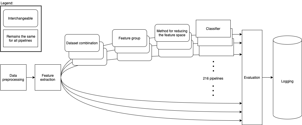
Figure 1 shows the outlines of the architecture we propose. The first step is data preprocessing, explained in Section 4.1. Preprocessed data is then fed to the feature extraction step explained in Section 4.2. Then we organize 216 separate pipelines that consist of unique combinations of datasets, feature groups, and methods for reducing the feature space explained in Section 4.3. All pipelines use the same ensemble classifier. Results are then evaluated in the evaluation step (see Section 4.4) and logged (see Section 4.5).
4.1. Preprocessing
This subsection explains how we achieved goals 1 & 2 of creating a platform for generating generalizable features.
We need methods to standardize datasets so the units are the same and the data is in the same form.
We need to clean the data to achieve high data quality, which can produce good features.
4.1.1. Standardization of Datasets
We use three datasets from different experiments with different contexts. Each dataset has its own set of column names, and they also use different units. Some of the datasets measure time in milliseconds, while others measure it in microseconds. In standardizing the dataset, we converted all differing units and renamed columns representing the same values so that all datasets are consistent. Some subjects were missing labels; this was solved by removing the subject from the dataset.
For the EMIP dataset, we were provided with the raw data without fixations calculated. In order to use this dataset, we calculated fixations ourselves with the library PyGaze Analyzer [78]. The algorithm used is a dispersion-based algorithm that requires us to set the maximum distance and minimum duration for a fixation. We set the minimum duration by finding the minimum duration of fixations from our two other datasets. Pieter Blignaut [79] suggests that the maximum distance of a fixation when using a dispersion algorithm for finding fixations should be 1º of the foveal angle. The distance between the subject and the stimulus was 700 mm for EMIP; thus, 1º of the foveal angle works out to about 45 pixels. We only used fixations where the subject was reading code and disregarded data gathered during setup and calibration.
4.1.2. Normalization and Outlier Removal
As our subjects come from multiple contexts, the need for normalization and outlier removal is extra apparent. It is essential to normalize pupil diameter. Pupil diameter can be affected by several factors, such as lighting conditions and how well-rested the subject is [80]. We chose to min-max normalize the pupil diameter in the range of 0 to 1 per subject. To mitigate some contextual biases, we use a rolling mean with a window size of 100 samples to smooth the timeseries.
Our time recordings are made at the start point of each fixation. This can be problematic, as there are situations where more time passes between fixations than would be reasonable for regular saccades. This might be due to blinking, the subject looking outside the range of the eye-tracker, or technical malfunction. To mitigate this, we remove the outliers by setting a threshold of 1000 ms for saccade duration. All gaps in time over 1000ms were reduced to 1000ms.
4.2. Feature Extraction
This subsection explains how we achieved goal 3.
We need a platform that can generate computationally expensive features for multiple large datasets.
We will present the flow of the feature extraction process and discuss the specific features we extract. The features are organized into three sections:
-
Timeseries Features
-
Gaze Characteristics
-
Heatmap features
4.2.1. Flow
The flow of the feature extraction job is as follows:
-
Download the datasets from google cloud storage.
-
Standardize and normalize data.
-
Generate aggregated attributes, such as saccade duration and saccade_length.
-
Smooth the signal with rolling mean.
-
Generate features.
-
Upload features to google cloud storage.
4.2.2. Timeseries Features
After preprocessing, our dataset includes several different eye-tracking variables. The variables we use are pupil diameter, fixation duration, saccade duration, and saccade length. We interpret these signals with different timeseries modeling techniques, which are elaborated upon in this section.
From each of these signals, we calculate five features.
-
Power Spectral Histogram.
-
ARMA.
-
GARCH.
-
Hidden Markov Models.
-
LHIPA.
Power Spectral Histogram
The power spectrum decomposes the timeseries into the frequencies in the signal and the amplitude of each frequency. Once computed, they can be represented as a histogram called the power spectral histogram. We computed the centroid, variance, skew, and kurtosis of the power spectral histogram.
The power spectral histogram describes the repetition of patterns in the data. We hypothesize that similar pattern repetitions will be present in subjects that display a high cognitive performance across contexts.
Autoregressive Moving Average model (ARMA)
We know that a cognitive process takes place over a span of time, and our gaze data is organized as a timeseries. If our goal is to model cognitive workload, we need to capture the temporal aspects of cognition. ARMA combines an auto-regressive part and a moving average part to model movements in a timeseries. It uses information for previous events to predict future events with the same source.
An ARMA process describes a time series with two polynomials. The first of these polynomials describes the autoregressive (AR) part of the timeseries. The second part describes the moving average (MA). The following formula formally describes ARMA:
\$X_t = sum_(j=1)^p phi_j X_(t-j) + sum_(i=1)^q theta_i epsilon_(t-i) + epsilon_t\$
The features we extract from ARMA are extracted with the following algorithm
best_fit = null
for p up to 4
    for q up to 4
        fit = ARMA(timeseries, p, q)
        if(best_fit.aic > fit.aic)
            best_fit = fit
return best_fit["ar"], best_fit["ma"], best_fit["exog"]
Generalized AutoRegressive Conditional Heteroskedasticity (GARCH)
GARCH is similar to ARMA, but it is applied to the variance of the data instead of the mean.
ARMA assumes a uniform distribution of the events it is modeling with shifting trends. However, we know that this is not entirely descriptive of cognitive processes. When working with a cognitive task, one has periods of intense focus to understand one aspect of the problem and other periods where one’s mind rests. The heteroskedasticity aspect of GARCH accounts for this grouping of events. In the analysis of financial markets, GARCH can account for the spikes and sudden drops in prices of specific investment vehicles [81]. We posit that GARCH will allow us to model the perceived grouping of cognitive workload spikes in a like manner.
We extract features from GARCH similar to how we extract features from ARMA.
best_fit = null
for p up to 4
    for q up to 4
        fit = GARCH(timeseries, p, q)
        if(best_fit.aic > fit.aic)
            best_fit = fit
return [best_fit["alpha"],
       best_fit["beta"],
       best_fit["gamma"],
       best_fit["mu"],
       best_fit["omega"]]
Hidden Markov Models (HMM)
Hidden Markov Models contains the Markov assumption, which assumes that the present value is conditionally independent on its non-ancestors given its n last parents. Similarly to ARMA, this means that the current value is a function of the past values. While ARMA models continuous values, HMM is discrete. Hence we discretize the values into 100 buckets before we model the transitions between these buckets with HMM. We then use the resulting transition matrix as the feature.
The reasoning behind using HMM is the same as to why we chose ARMA. We hypothesize that HMM might model the changing state nature of cognitive work.
normalized_timeseries = normalize the timeseries between 0 and 1
discretized_timeseries = discretize timeseries in 100 bins
best_fit = null
for i up to 8
   fit = GaussianHMM(covariance_type="full")
        .fit(discretized_timeseries, n_components=i)
   if(best_fit.aic > fit.aic)
        best_fit = fit
flat_transistion_matrix = best_fit.transition_matrix.flatten()
padded_transition_matrix =
    pad flat_transistion matrix with n zeroes so the length is 64
return padded_transition_matrix
The Low/High Index of Pupillary Activity (LHIPA)
LHIPA [13] enhances the Index of Pupillary Activity [14], which is a metric to discriminate cognitive load from pupil diameter oscillation. LHIPA partially models the functioning of the human autonomic nervous system by looking at the low and high frequencies of pupil oscillation.
Cognitive load has been shown to correlate with cognitive performance [82]. The Yerkes-Dodson law describes the relationship between the two, indicating an optimal plateau where a certain degree of cognitive workload is tied to maximized cognitive performance. If the cognitive workload is increased beyond this point, cognitive performance is diminished [82].
4.2.3. Gaze Characteristics
Gaze Characteristics are features that are interpreted directly from the eye-tracking data and are not subject to additional signal processing.
Information Processing Ratio
Global Information Processing (GIP) is often analogous to skimming text. When skimming, one’s gaze jumps between large sections of the material and does not stay in place for extended periods. This manifests as shorter fixations and longer saccades. Local Information Processing (LIP) is the opposite; one’s gaze focuses on smaller areas for longer durations and does not move around as much. For this metric, fixations are measured in time, while saccades are measured in distance. Hence we capture both the spatial and temporal dimensions.
The information processing ratio describes how much a subject skimmed the material versus how much they focus intently. To compute the ratio, we divide GIP by LIP.
The following algorithm extracts the feature:
upper_threshold_saccade_length = 75 percentile of saccade_lengths
lower_threshold_saccade_length = 25 percentile of saccade_lengths
upper_threshold_fixation_duration = 75 percentile of fixation_durations
lower_threshold_fixation_duration = 25 percentile of fixation_durations

LIP = 0
GIP = 0
for s_length, f_duration in saccade_lengths, fixation_durations
    fixation_is_short = f_duration <= lower_threshold_fixation_duration
    fixation_is_long = upper_threshold_fixation_duration <= f_duration
    saccade_is_short = s_length <= lower_threshold_saccade_length
    saccade_is_long = upper_threshold_saccade_length <= s_length

    if fixation_is_long and saccade_is_short:
        LIP += 1
    elif fixation_is_short and saccade_is_long:
        GIP += 1

return GIP / (LIP + 1)
Skewness of Saccade Speed
Saccade velocity skewness has been shown to correlate with familiarity [83]. If the skewness is highly positive, that means that the overall saccade speeds were high. This indicates that the subject is familiar with the stimulus and can quickly maneuver to the relevant sections when seeking information. Saccade speed does not necessarily indicate expertise in the relevant subject matter. A non-expert participant could be familiar with the material and hence know where to look for information, but an expert would also quickly assert what information they are seeking.
To calculate this feature, we calculated the speed by dividing the saccade length by the saccade duration. We then got the skew of the outputted distribution.
get_skewness_of_saccades(saccade_duration, saccade_length):
    saccade_speed = saccade_length / saccade_duration
    return saccade_speed.skew()
Verticality of Saccades
By verticality of saccades, we mean the ratio of saccades moving vertically over horizontally. Our intuition for generating this feature is based on the difference between how we read code versus how we read text. An experienced coder reads vertically, focusing on definitions and conditionals. Traditional text, on the other hand, is read line by line in a horizontal fashion. Based on this anecdotal observation, we are interested in how well the verticality of saccades would generalize.
To calculate the feature, we get the angle between every consecutive fixation with respect to the x-axis. We do that with arctan2, which outputs the angle in radians between pi and -pi. Since we are only interested in the verticality of the saccade, we take the absolute value of the angle. To describe the horizontality of each point in a range between 0 and 1, we take the sine of every angle.
angles = atan2(y2 - y1, x2 - x1)

for angle in angles
   angle = sin(absolute_value(angle))

verticality = angles.average()
Entropy of Gaze
The entropy of gaze explains the size of the field of focus for a subject. Entropy is higher when the subject’s attention is more evenly spread over the stimulus and lower if the subject focuses on a minor part of the stimulus.
To calculate the entropy of gaze, we create a grid of 50 by 50 px bins. We then normalize the x and y positions of each fixation in a range from 0 to 1000. Further, we place each fixation in its corresponding bin based on its x and y position. When we have this grid, we flatten it and take the entropy of the resulting distribution.
The following algorithm extracts the feature:
x_normalized = normalize x between 0 and 1000
y_normalized = normalize y between 0 and 1000

x_axis = [50, 100, 150 ... ,1000]
y_axis = [50, 100, 150 ... ,1000]
2d_histogram = 2d_histogram(xaxis, yaxis, x_normalized, y_normalized)
return entropy(2d_histogram.flatten())
4.2.4. Heatmaps
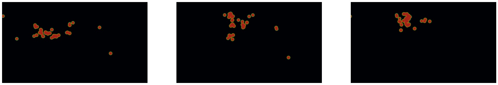
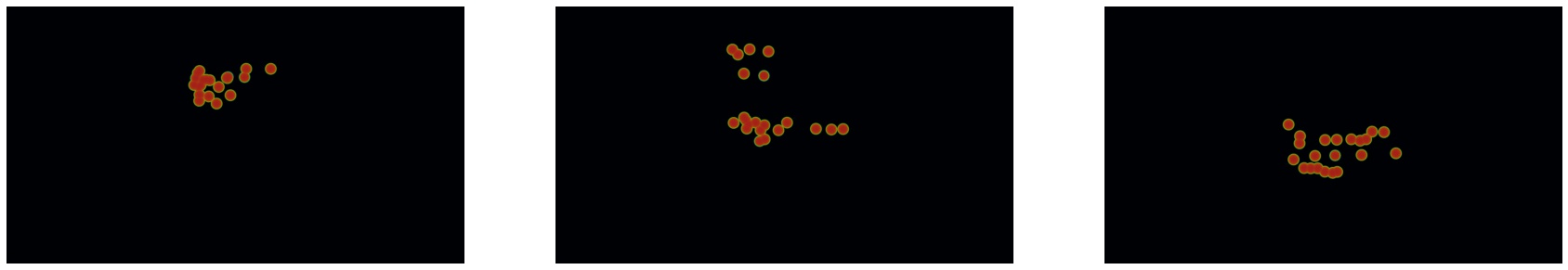
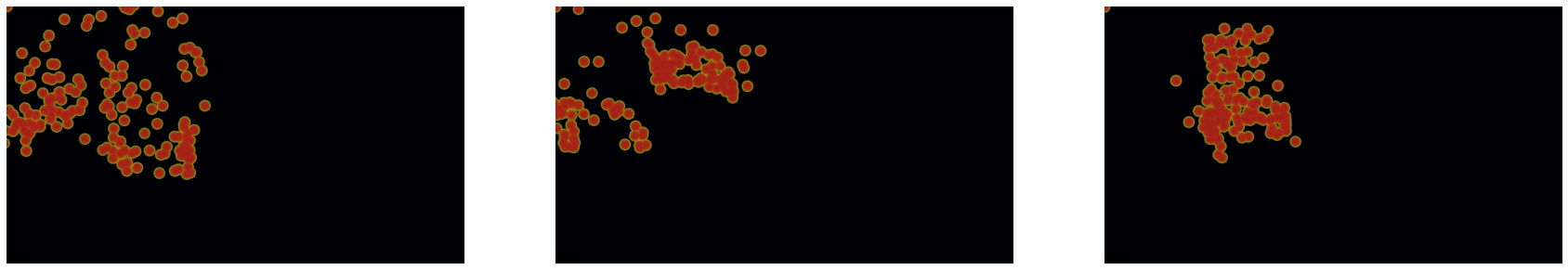
A heatmap is a graphical representation of data where values are depicted by color. Areas of higher activity will be highlighted more. Our heatmaps represent the gaze position of a subject over time. To capture both spatial and temporal data, we create multiple heatmaps for each subject. Sharma et al. [34] show that deep features of heatmaps from gaze data can predict cognitive performance in learning activities.
These are the steps we take to create our heatmaps:
-
Split the data from each subject into 30 partitions.
-
Create a 1920 * 1080 image.
-
Plot the gaze position with heatmappy [84].
-
Resize the image to 175 * 90.
From the heatmaps, we used a pre-trained vgg19 model [85] with the imagenet weights [86] to generate a feature vector per image.
-
Scale images using the preprocess_input function provided by Keras [87]
-
Use the pre-trained VGG-19 model to extract features per image
-
Combine the matrices outputted by the VGG19 model to a single feature vector
frames = Split each subject into 30 partitions
features = []
for frame in frames
    image = image of with dimensions 1920, 1080
    heatmap = heatmappy.heatmap_on_img(frame.x_and_y_postions, image)
    scaled_down_heatmap = keras.applications.image_netutils(heatmap)
    heatmap_features = vgg19model.predict(scaled_down_heatmap)
    features.append(heatmap_feature.flatten())
return features.flatten()
4.2.5. Final Feature Set
After feature extraction, these are the features that are generated for each subject.
| Name | Description |
|---|---|
Information Processing Ratio |
LIP divided by GIP. |
Saccade Speed Skewness |
Skewness of the saccade speed distribution. |
Entropy of Gaze |
Entropy of the gaze |
Verticality Of Saccades |
Metric between 0 and 1 describing the average angle of the saccades. |
Heatmaps |
Features extracted from heatmaps with VGG19. |
Spectral Histogram - Pupil Diameter |
Skew, Kurtosis, Mean, and Variance of the spectral histogram. |
LHIPA - Pupil Diameter |
The Low/High Index of Pupillary Activity. |
HMM - Pupil Diameter |
Transition matrix of a fitted Hidden Markov Model. |
ARMA - Pupil Diameter |
The AR, MA, and Exog attributes of a fitted ARMA model. |
GARCH - Pupil Diameter |
The mu, omega, alpha, gamma, and beta attributes of a fitted GARCH model. |
Spectral Histogram - Fixation Duration |
Skew, Kurtosis, Mean, and Variance of the spectral histogram. |
HMM - Fixation Duration |
Transition matrix of a fitted Hidden Markov Model. |
ARMA - Fixation Duration |
The AR, MA, and Exog attributes of a fitted ARMA model. |
GARCH - Fixation Duration |
The mu, omega, alpha, gamma, and beta attributes of a fitted GARCH model. |
Spectral Histogram - Saccade Length |
Skew, Kurtosis, Mean, and Variance of the spectral histogram. |
HMM - Saccade Length |
Transition matrix of a fitted Hidden Markov Model. |
ARMA - Saccade Length |
The AR, MA, and Exog attributes of a fitted ARMA model. |
GARCH - Saccade Length |
The mu, omega, alpha, gamma, and beta attributes of a fitted GARCH model. |
Spectral Histogram - Saccade Duration |
Skew, Kurtosis, Mean, and Variance of the spectral histogram. |
HMM - Saccade Duration |
Transition matrix of a fitted Hidden Markov Model. |
ARMA - Saccade Duration |
The AR, MA, and Exog attributes of a fitted ARMA model. |
GARCH - Saccade Duration |
The mu, omega, alpha, gamma, and beta attributes of a fitted GARCH model. |
4.3. Pipelines
This section explains how we solved goal 4 of creating our platform.
We need a platform that can run multiple concurrent pipelines for combinations of datasets, features, and methods for reducing the feature space.
By a pipeline, we mean a specific combination of datasets, feature groups, and methods for reducing the feature space (dimensionality reduction or feature selection). We will refer to these parts as pipeline components.
4.3.1. Datasets
We have three different datasets: EMIP, Fractions, and CSCW. As discussed in Section 3, we designate either one or two datasets as in-study for each of our pipelines. All pipelines include a single dataset as the out-of-study dataset. No dataset is used twice in one pipeline.
We refer to the pipelines where one dataset is designated in-study as 1-to-1 pipelines, as these pipelines train on one dataset and test on another. Pipelines, where two datasets are designated in-study, are referred to as 2-to-1 pipelines since we train on two datasets combined and test on one dataset. We have three datasets, which make up nine dataset combinations, six of which create 1-to-1 pipelines, and three go into 2-to-1 pipelines.
4.3.2. Feature Groups
Initially, we considered running pipelines to test all combinations of features. These would prove to be unfeasible. With 22 features, nine dataset combinations, and two methods of reducing the feature space, there would be 75 597 472 pipelines. With a theoretical runtime of one second per pipeline, the total computing time necessary to tackle this challenge would be approximately two years, and we would not make our deadline for this thesis.
As an alternative, we decided to group our features manually. We created one group for the gaze characteristics, four for the type of signal, and five for the different time series features. In addition, we have a separate group for heatmaps and, lastly, one group that includes all the features. The groups are presented in the following table:
| Name | Features |
|---|---|
Gaze Characteristics |
Information Processing Ratio, |
Heatmaps |
Heatmaps |
Spectral Histogram |
Spectral Histogram - Pupil Diameter, |
LHIPA |
LHIPA - Pupil Diameter |
HMM |
HMM - Fixation Duration, |
ARMA |
ARMA - Pupil Diameter, |
GARCH |
GARCH - Saccade Duration, |
Pupil Diameter |
Spectral Histogram - Pupil Diameter, |
Fixation Duration |
Spectral Histogram - Fixation Duration, |
Saccade Length |
Spectral Histogram - Saccade Length, |
Saccade Duration |
Spectral Histogram - Saccade Duration, |
All |
All features |
4.3.3. Reducing the Feature Space
Our pipelines perform either feature selection or dimensionality reduction to reduce the number of features and decrease variance. The focus of our thesis was on testing different features, and as such, we decided not to test a wide range of alternatives. The effect of different methods for reducing the feature space on generalizability is a potential area for further study. The method we use for dimensionality reduction is Principal Component Analysis (PCA), and the one for feature selection is Least Absolute Shrinkage and Selection Operator (LASSO). We also use a zero-variance filter for all pipelines to remove the features with no variance in their data.
4.3.4. Prediction: Ensemble Learning
Our pipelines were tested with the same regressor, a weighted voting ensemble with a KNN-regressor, a Random forest regressor, and a Support Vector regressor. An ensemble combines several different base regressors or classifiers in order to leverage the strengths of each classifier or regressor. A voting regressor is an ensemble that fits several regressors, each on the whole dataset. Then it averages the individual predictions respective to their given weights to form a final prediction. To find the weights for the voting, we perform cross-validation, with the validation set, on each regressor and set their respective weights to 1 - Root Mean Square Error (RMSE). Many studies have been published that demonstrate that ensemble methods frequently improve upon the average performance of the single regressor [90, 91].
KNN predictors approximate the target by associating it with its n nearest neighbors in the training set. KNNs are simplistic algorithms that, despite their simplicity, in some cases, outperform more complex learning algorithms. However, it is also negatively affected by non-informative features [92]. A random forest fits a number of classifying decision trees on various sub-samples of the dataset and aggregates the predictions from the different trees. Random forests have been shown to outperform most other families of classifiers [93]. SVR, support vector regressors are a regression version of support vector machines proposed by Drucker et al. [94] SVRs estimate the target value by fitting a hyperplane by minimizing the margins of the plane with an error threshold. Support vector regressors perform particularly well when the dimensionality of the feature space representation is much larger than the number of examples [94], which is the case for some of our feature groups. All our hyperparameters are set to the default values provided by sklearn [95].
4.4. Evaluation
This section will outline how we achieve the fifth goal of our platform:
We need an evaluation step that collects the results from all the pipelines and can prove pipelines generalizable.
Models produced by our pipelines are evaluated in two ways, with out-of-sample testing and out-of-study testing. Out-of-sample testing uses a subset of the in-study dataset to evaluate the predictive power of the model. Out-of-study testing uses the dataset designated as out-of-study to evaluate generalizability. This subsection explains how we evaluate the results of each test.
4.4.1. Evaluation Criteria
We use Normalized Root Mean Squared Error (NRMSE) as our primary evaluation metric. NRMSE is a probabilistic understanding of errors as defined by Ferri et al. [96]. NRMSE is commonly used in learning technologies to evaluate learning predictions [97]. The score in all our contexts is based on binary outcomes; a question is either correct or incorrect. Pelánek et al. [98] argue that for such cases, metrics such as Root Mean Squared Error (RMSE) or Log-Likelihood (LL) are preferred to metrics such as Mean Average Error (MAE) or Area Under the Curve (AUC). MAE considers the absolute difference between the predictions and the errors and is not a suitable metric, as it prefers models that are biased toward the majority result. RMSE, on the other hand, does not have this issue, as it is based on the squared value of each error, giving greater weight to larger errors in its average. The main difference between RMSE and LL is the unbounded nature of LL, which means that it can very heavily punish models that confidently make incorrect assertions [98]. While this can be preferred in some contexts, we decided to proceed with the more common RMSE measure.
The root part of RMSE serves to move the sum of errors back into the range of the labels being predicted to improve interpretability. This might have limited usefulness as the resulting numbers can still be challenging to interpret [98]. In our case, the labels exist in three different contexts with labels in different ranges, and since we are working across these contexts, we need normalized values. Since we normalize the labels in a range from 0 to 1 before training, RMSE is equivalent to Normalized RMSE (NRMSE). Our NRMSE is normalized between 0 and 1, where 1 is the maximum error possible for the dataset.
The following formulas calculate NRMSE.
\$RMSE = sqrt ((sum_(i=1)^text(Number of samples) (text(predicted)_i - text(original)_i)^2) / text(Number of Samples))\$
\$NRMSE = text(RMSE)/(text(original)_max - text(original)_min)\$
4.4.2. Feature Generalizability Index (FGI)
Our measure for generalizability was proposed by Sharma et al. [24]. We measure the generalizability of features by comparing the distributions of NRMSE values from the out-of-sample testing and the out-of-study testing. Since the ground truth in both the in-study datasets and the out-of-study datasets indicate cognitive performance, we can assume that similar behavior will indicate similar results. To compare the distributions of NRMSE, we use analysis of similarity (ANOSIM), a non-parametric function, to find the similarity of two distributions [99].
\$(text(mean ranks between groups ) - text( mean ranks within groups))/(N(N - 1)/4)\$
The denominator normalizes the values between -1 and 1, where 0 represents a random grouping. Pipelines that have an FGI value closer to zero are more generalizable [24].
4.5. Reproducibility
This section explains how we reached the sixth goal of our platform.
We need reproducibility.
Our reproducibility strategy primarily consists of four components. The version-control tool, git; the machine learning management tool, comet.ml; the python package management tool, poetry; and google cloud platform.
4.5.1. comet.ml
comet.ml is a machine learning management tool [100]. It can handle user management, visualization, tracking of experiments, and much more. We use comet.ml to track the results of our experiments, the relevant hyperparameters, the git commit hash, which indicates our software state, and the virtual machine on the google cloud platform, which executed the code.
4.5.2. Poetry
Poetry is a dependency manager for python [101]. As with any large software project, our platform relies on several third-party libraries. To ensure both reproducibility and ease of use and development, we use poetry to track the versions of the libraries we use. Poetry stores these versions in a lock-file which is tracked by git.
4.5.3. Git
Git keeps track of all versions of our source code [102]. We have set up safeguards that ensure that all changes to the local code are committed before a run can begin. In addition, all parameters of experiments are represented in the code. As a result, the complete state of the software, including configuration and hyper-parameters, is recorded in git. The commit hash, which uniquely identifies the point of commitment in our history, is logged, and we can reproduce the software side of our experiment.
When we run an experiment in the cloud, we log the start parameters of the system and the hash associated with the commit.
4.5.4. Google Cloud Platform
Our experiments are run on virtual machines in the Google Cloud Platform (GCP) [103]. GCP is one of several providers of commercial cloud and containerization services. Their products allow us to run our experiments on identical virtual machines, which also ensures reproducibility in our work’s hardware aspects.
4.5.5. Seeding
All of our experiments ran with seeded randomness. Our implementation for seeding the experiments is as follows:
seed = 69420
np.random.seed(seed)
random.seed(seed)
os.environ["PYTHONHASHSEED"] = str(seed)
tf.random.set_seed(seed)
4.5.6. Datasets
At this point, we can reproduce any of the experiments presented in this work. However, as we cannot share the data we received from other researchers, complete external repeatability is impossible.
5. Results
We ran a total of 216 pipelines with different combinations of datasets, methods for reducing the feature space, and feature groups. 144 of these pipelines were 1-to-1 pipelines, where we trained on only one dataset and tested on another. 72 of the pipelines were 2-to-1, where two datasets are designated in-study and one dataset designated out-of-study. In this section, we will present the results from these pipelines. In Section 5.1, we explain how baselines for the different datasets are calculated. Section 5.2 presents how pipelines performed in out-of-sample testing and which components performed the best overall by aggregating the results. The pipelines that show generalizability are presented in Section 5.3. The section also presents which components make up those pipelines. Pipelines that exhibit more context-sensitivity are presented in Section 5.4.
5.1. Baselines
We calculate a specific baseline for each dataset combination. The baseline is equivalent to predicting the mean of the labels from the in-study dataset. We then quantify this baseline by the NRMSE from those predictions. The calculation of the baseline is done separately for each dataset combination. Our pipelines are evaluated against the baseline for the given dataset combination.
| Dataset | Baseline (NRMSE) |
|---|---|
CSCW |
0.205 |
EMIP |
0.310 |
Fractions |
0.229 |
EMIP & Fractions |
0.294 |
EMIP & CSCW |
0.289 |
CSCW & Fractions |
0.234 |
Pseudocode for the in-study baseline:
def get_baseline(labels):
    error = labels - labels.mean()
    error_squared = (error**2).mean()
    baseline = math.sqrt(error_squared)
    return baseline
5.2. Out-of-Sample Testing
Our work focuses on engineering generalizable features. This section outlines the results from the out-of-sample testing, which does not indicate generalizability. However, the section is presented to the reader to benchmark the range of predictive power that our features exhibit in more traditional tasks.
5.2.1. Aggregation of the Results
To evaluate how each feature space reduction method and each feature combination performs across all the pipelines, we need to aggregate the pipelines' results. We do this by ranking, giving each pipeline a rank for NRMSE, then grouping on feature space reduction method or feature group, and finding the median. The median of ranks gives us the results of what pipeline components perform best when testing in the same context it was trained.
5.2.2. Dimensionality Reduction and Feature Selection
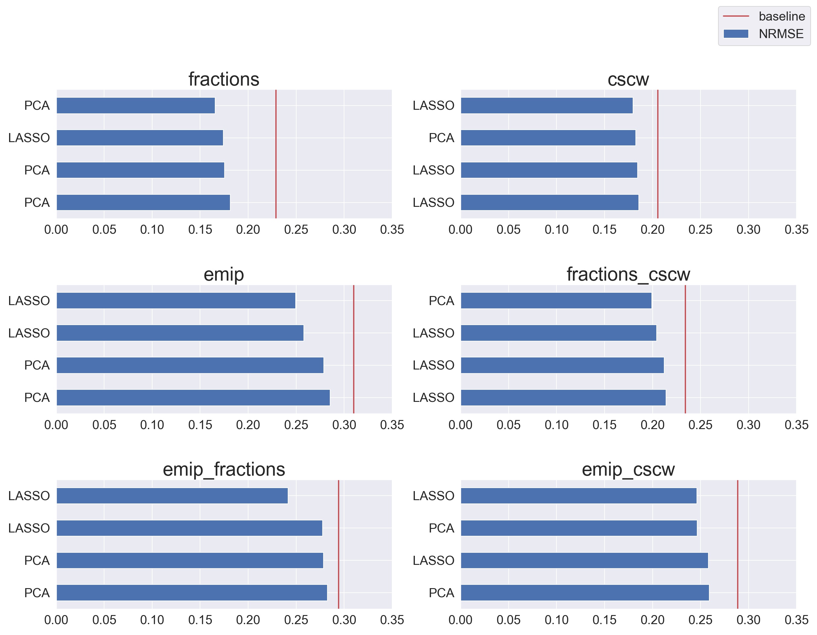
Figure 5 shows which method reduces the feature space for the pipelines with the five smallest NRMSEs per dataset. Which method performs better seems to rely heavily on the in-study dataset, making it hard to conclude which of the two performs better.
However, when we aggregate the results as seen in Table 4 and Table 5, we can see that LASSO performs slightly better than PCA across all 1-to-1 pipelines and clearly better across the 2-to-1 pipelines. So our results indicate that feature selection performs better than dimensionality reduction in predicting cognitive performance on gaze data for out-of-sample testing.
| Method | Mean NRMSE | Median NRMSE Rank |
|---|---|---|
LASSO |
0.265 |
69.5 |
PCA |
0.269 |
76.0 |
| Method | Mean NRMSE | Median NRMSE Rank |
|---|---|---|
LASSO |
0.272 |
31.5 |
PCA |
0.283 |
44.0 |
5.2.3. Features
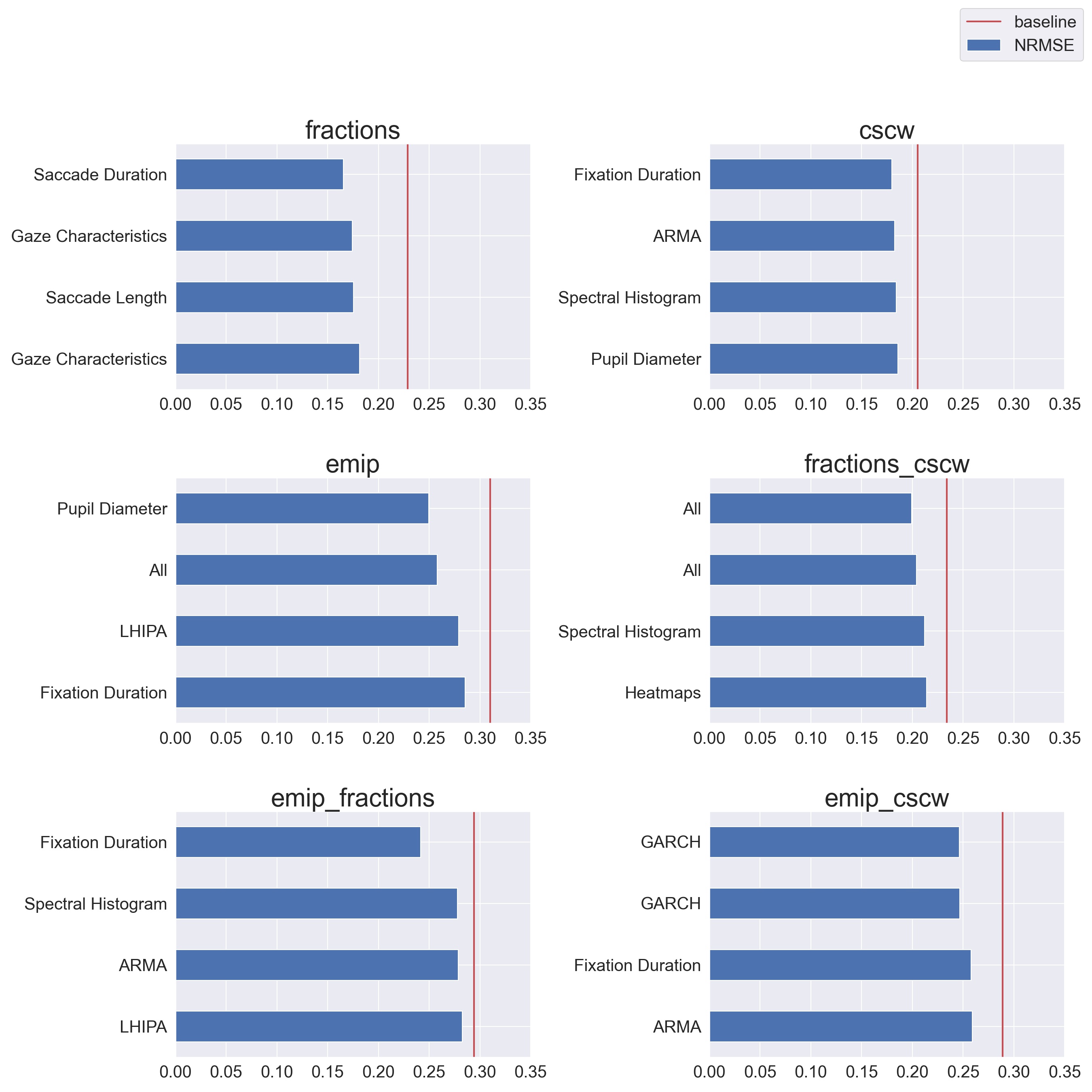
Figure 6 shows the best four pipelines by NRMSE and their feature groups. It seems that several different feature groups perform quite well for the different dataset combinations. We note that Fixation duration performs well in most combinations and that Spectral Histograms performs well in several pipelines, and All perform well, particularly for fractions_cscw.
As seen in Table 6 and Table 7, when we aggregate the results, we see that Gaze Characteristics is the best feature group for out-of-sample testing amongst the 1-to-1 pipelines, performing slightly better than Spectral Histograms and Heatmaps. 2-to-1 pipelines that include Fixation duration seem to outperform other 2-to-1 pipelines, but GARCH also performs quite well.
| Method | Mean NRMSE | Median NRMSE Rank |
|---|---|---|
Gaze Characteristics |
0.246 |
34.0 |
Spectral Histogram |
0.268 |
45.0 |
Heatmaps |
0.253 |
51.0 |
Pupil Diameter |
0.274 |
63.5 |
Saccade Length |
0.266 |
65.0 |
| Method | Mean NRMSE | Median NRMSE Rank |
|---|---|---|
Fixation Duration |
0.269 |
22.5 |
GARCH |
0.264 |
24.0 |
Spectral Histogram |
0.271 |
31.5 |
All |
0.267 |
32.5 |
LHIPA |
0.282 |
37.5 |
5.3. Generalizability
We evaluate the generalizability of the pipelines with the out-of-study dataset. We compare the errors from making predictions on the out-of-study dataset to the out-of-sample results using FGI, explained in Section 4.4.2. In order to identify the most generalizable pipelines, we need to filter out pipelines that perform poorly in out-of-sample testing. We do this by filtering out the pipelines that do not perform better than the baseline. From 216 pipelines, 72 beat the baseline.
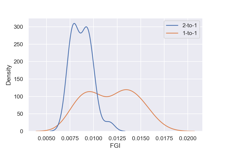
As represented in Figure 7, 2-to-1 pipelines are, in general, more generalizable than 1-to-1 pipelines. This is in line with the results of [24]. Our focus is generalizability, and as such, we will only refer to the 2-to-1 pipelines in the following sections.
| FGI | In Study | Feature Group | PCA or LASSO |
|---|---|---|---|
0.007 |
fractions_cscw |
GARCH |
LASSO |
0.0074 |
fractions_cscw |
Spectral Histogram |
LASSO |
0.0074 |
fractions_cscw |
All |
PCA |
0.0077 |
fractions_cscw |
Saccade Duration |
LASSO |
0.0077 |
fractions_cscw |
Heatmaps |
PCA |
0.0077 |
fractions_cscw |
Saccade Length |
LASSO |
0.0077 |
fractions_cscw |
Heatmaps |
LASSO |
0.0078 |
fractions_cscw |
All |
LASSO |
0.0078 |
fractions_cscw |
HMM |
LASSO |
0.0081 |
emip_cscw |
GARCH |
PCA |
Table 8 shows the most generalizable pipelines. The first and most prevalent factor for generalizable pipelines is which datasets were designated in-study datasets for that pipeline. When the in-study dataset combines Fractions and CSCW (fractions_cscw), and EMIP is the out-of-study dataset, the pipelines are more generalizable. Nine of the ten more generalizable pipelines contain this combination of datasets.
LASSO is the most represented method of feature space reduction among the more generalizable pipelines. We note that more pipelines with LASSO beat the baseline, which might explain the trend we are seeing. LASSO is also included in the two pipelines with the best FGI. PCA performs very well for the feature groups All and heatmap; this might be explained by the fact that these are the largest feature groups with hundreds of thousands of values.
Seven of our twelve feature groups are represented among the ten most generalizable pipelines. However, three feature groups show up more than once, All, Heatmaps, and GARCH. This indicates that they might be more generalizable feature groups. It should also be noted that GARCH is also the only pipeline with an in-study dataset that is not fractions_cscw of the ten most generalizable pipelines.
5.4. Context-Sensitivity
The bottom third of the filtered baselines contain pipelines that are more context-specific.
| FGI | In Study | Feature Group | PCA or LASSO |
|---|---|---|---|
0.0117 |
emip_cscw |
All |
LASSO |
0.0102 |
emip_cscw |
Gaze Characteristics |
LASSO |
0.0102 |
emip_cscw |
Pupil Diameter |
LASSO |
0.0098 |
emip_cscw |
Saccade Length |
LASSO |
0.0096 |
emip_cscw |
HMM |
LASSO |
0.0096 |
emip_fractions |
LHIPA |
PCA |
0.0095 |
emip_fractions |
Spectral Histogram |
LASSO |
0.0093 |
emip_cscw |
Heatmaps |
LASSO |
0.0093 |
emip_cscw |
ARMA |
PCA |
Again we can see that the dataset combination is an important factor in what pipelines exhibit context-sensitivity. LASSO is more represented among the more context-specific pipelines. As with the generalizable pipelines, there are more pipelines with LASSO that beat the baseline. For the feature groups, we observe some differences from the generalizable pipelines. ARMA, LHIPA, Gaze Characteristics, and Pupil Diameter are present in the context-sensitive pipelines but not in the more generalizable pipelines. This indicates that these feature groups are more likely to produce context-sensitive pipelines. Heatmaps, Spectral Histogram, Hidden Markov Models, All, and Saccade Length appear in generalizable and context-sensitive pipelines. This further supports the observation that dataset combination is an essential variable for generalizability.
6. Discussion
6.1. Findings
-
2-to-1 pipelines are more generalizable than 1-to-1 pipelines.
-
2-to-1 pipelines where Fractions and CSCW are the in-study datasets produce more generalizable pipelines.
-
GARCH, Power Spectral Histogram, heatmaps, Saccade Duration, Saccade Length, and HMM can produce generalizable pipelines.
-
Pupil Diameter, Gaze Characteristics, LHIPA, and ARMA, can produce context-sensitive pipelines, and we do not observe any tendencies to generalize.
6.2. Filtering on the Baseline
Our goal was to identify generalizable pipelines, and for that, we have the FGI measure described in Section 4.4.2. FGI describes how similar the distribution of errors from out-of-sample testing and out-of-study testing and is a measure of generalizability [24]. However, it is not enough that the two distributions are similar. Generalizability should be a measure of usable predictive power in contexts other than the training context. Random guesses would create identical distributions of error in out-of-sample testing and out-of-study testing, and as such, would have a good FGI value. To counteract this, we chose to disregard all pipelines that do not outperform their respective baselines for the purpose of measuring generalizability.
6.3. 2-to-1 versus 1-to-1
As shown in Figure 7, 2-to-1 pipelines tend to generalize better than 1-to-1 pipelines. Combining two datasets from two separate contexts for training introduces more variability to the dataset. By introducing more variability, we are optimizing for both bias and variance, which is crucial for generalizability [48]. These results align with the findings of Sharma et al. [24]. When we generate a feature that can predict cognitive performance in two separate contexts, that feature has mutual information with cognitive performance in those two contexts. Such a feature likely describes some non-contextual aspects of cognitive performance, meaning it should have higher mutual information with cognitive performance in a third context. In further discussions, we will focus on results from the 2-to-1 pipelines.
6.4. Generalizability of our Datasets
Table 8 indicates that pipelines that combine Fractions and CSCW for training and use EMIP for testing are more generalizable than pipelines where EMIP was included in the training set. The EMIP dataset consists of gaze data recorded of people completing individual tasks. All datasets include information from one or more context-specific tasks, but the Fractions and CSCW also have a collaborative aspect. We theorize that pipelines trained on EMIP do worse at describing this collaborative aspect. The variability introduced by the interactions that come with collaborative work assists those pipelines in generalizing. There is a degree of division of labor in collaboration, which gives rise to individual tasks even in the collaborative context; as such, there is mutual information even with cognitive performance in individual tasks even when training on collaborative tasks. Pinpointing the effectiveness of training on collaborative data when generalizing to contexts without a collaborative aspect is a promising area for more experimentation.
6.5. Generalizable Features
Table 8 presents our more generalizable pipelines. In this section, we will explain why we believe the feature groups used in those pipelines generalize.
6.5.1. Heatmaps
We observe that Heatmaps are among the generalizable feature groups. The feature group only contains one feature vector, the heatmaps. Our heatmap feature is the gaze-position for each subject over time, split into 30 partitions, converted to a heatmap, and fed to a pre-trained VGG19 model. The resulting feature vector is the feature we call heatmaps. In a heatmap, the stimulus is captured through the subject’s interaction with it, as the gaze pattern follows the stimulus. While the stimulus is not included in the heatmap image, information about the stimulus is still encoded. The feature vector we call heatmaps represents how the gaze interacts with the given stimulus. Taking EMIP as an example, a heatmap will tell us the shape of the code being presented to the subject. However, it will also tell us how much time a subject spends reading the syntactic structures versus the variable names or conditional logic. The latter two are focus points for experienced coders. Heatmaps generalize well because instead of just capturing how a subject interacts with their stimulus, it also captures their interaction patterns and how they relate to their presented stimulus. The stimulus and the interaction pattern individually might be context-specific; however, the relationship between the two should generalize. In addition, heatmaps encode information about time and space rather than just one of the dimensions.
6.5.2. GARCH and Spectral Histogram
GARCH is a statistical modeling technique used to model timeseries data. Our data suggest that GARCH is the most generalizable feature group of the ones we have tested. GARCH models the variance of data and has the heteroscedasticity property. Heteroscedasticity means that the random disturbance is different across the elements. In our case, this means the variance of indicators of cognitive performance varies from point to point in the timeseries. In different contexts, the timing of the indicators will vary based on the task and other factors. This might explain why GARCH is generalizable across contexts.
Our results indicate that spectral histograms generalize quite well. Spectral histograms are the distribution of frequencies and their corresponding amplitudes. Spectral histograms capture repetitiveness and hence might capture patterns of behavior exhibited by the subjects. Repetitiveness indicates a flow that suggests that the subject is comfortable in their task; on the other hand, chaotic non-repetitive behavior might occur when one is not comfortable. We suggest that this relationship should be represented across contexts and could be why spectral histograms seem to generalize.
6.5.3. Saccade Duration and Saccade Length
Both saccade duration and saccade length seem to generalize. Saccades are the movements of the eyes from one fixation to another. As discussed in Section 4.2.3.2, higher saccade speeds correlate with familiarity with the stimulus [83]. Saccade speed is a function of saccade duration and saccade length; both factors map familiarity to some degree. The fact that saccade duration and saccade length generalizes might be explained by the fact that familiarity with the interface is relevant for all tasks contained by our datasets. Table 9 shows that saccade length also displays context-sensitivity in some pipelines. De Luca et al. [28] show that saccadic length increases when reading longer pseudowords. Due to human limitations on how quickly an eye can move, saccade length and saccade duration will correlate after a certain threshold of saccade velocity is met. Reading code is analogous to reading pseudowords, which might explain why saccade length displays context-sensitivity when EMIP is one of the designated in-study datasets.
6.5.4. All
In pipelines with the All feature group, we combine all features in one group. Our results show that these pipelines capture both generalizable patterns and context-sensitive, as seen in Table 8 and Table 9. The feature preferred by the regressor will be the feature with the most mutual information with cognitive performance in the in-study datasets; when this feature also has mutual information with cognitive performance in the out-of-study dataset, the pipeline can generalize. Since the All feature group contains all the features, the generalizability of the pipeline is highly dependent on the selected in-study dataset Section 6.4. As a result, we see pipelines with the All feature group both among the most generalizable and the most context-specific pipelines.
6.6. Context-Specific Features
Table 9 presents our more context-sensitive pipelines. In this section, we will explain why we believe the feature groups exhibit context-sensitivity.
6.6.1. ARMA
Our results indicate that ARMA produces quite context-sensitive pipelines. ARMA models the conditional mean of a timeseries, as opposed to the variance which GARCH models. Intuitively the mean value would be more dependent on the measurement’s context than the variance. For example, an ARMA model would be impacted by a stimulus with longer distances between points of interest when modeling saccade length, while GARCH would not.
6.6.2. LHIPA and Pupil Diameter
LHIPA was developed to be an indicator of cognitive load [13]. Cognitive load consists of intrinsic, extraneous, and germane loads [10, 11, 12]. The characteristics of the material determine intrinsic and extraneous cognitive load. Intrinsic load is determined complexity of the information and extraneous load by the presentation of the material. Both of these are context-specific factors. On the other hand, the germane load is concerned with the subject’s personal characteristics and would likely be more generalizable. Our observations that LHIPA can produce context-sensitive pipelines indicate that LHIPA captures germane cognitive loads to a lesser degree.
Pupil diameter has been shown to be affected by several task-specific factors. Both task difficulty and time limits have an impact on pupil dilation [9]. These are task-related factors, and as such, it might explain why pupil diameter seems to produce context-specific pipelines.
Shojaeizadeh et al. also point out that pupil size might convey information about variation in cognitive effort. This factor seems more likely to generalize and is what we model with GARCH. GARCH of pupil diameter is included in this feature group. However, the group primarily consists of features that model the mean of the pupil diameter.
6.6.3. Gaze Characteristics
Gaze Characteristics is the group of features that are interpreted directly from the eye-tracking data and are not subject to additional signal processing. The feature group tries to encapsulate different strategies for interacting with the stimulus. The information processing ratio represents the tendency to skim text versus more focused reading. A skimming or focused reading strategy might be more appropriate for a specific task, which might be why this indicates context-specificity. However, this is not an entirely specific trait. There might be some skill involved in picking the correct strategy when presented with a stimulus, and greater familiarity might lead to a faster transition to focused reading.
Entropy models the spread of the gaze over the stimulus, which might model the generalizable aspect of focus; however, it is also affected by the task design. The verticality of saccades is also certainly context-specific as it relies heavily on the nature of and how the stimulus is organized.
6.7. Limitations and Further Work
In Section 3.2, we outline how we believe our datasets are representative of a significant portion of human cognition. However, it would be presumptuous to say that three datasets from three different contexts could represent all of the cognitive processes. Our goal has been to generalize between our three contexts, and we believe that our methods provide meaningful insights into how one could create generalizable features for other contexts. We do not mean to say that our features will generalize to any context. Nevertheless, this is a first step that provides evidence on how gaze-related features provide a certain level of generalizability across three distinct and commonly employed contexts.
Table 8 and Table 9 show some indications that datasets from individual tasks generalize poorly to contexts that include collaborative work. Had individual work been better represented in our data, we might be able to say more about how individual tasks generalize in general. Ideally, we should have had at least one more dataset for individual tasks.
Our work assumes that cognitive performance can be characterized by labels in our datasets and represented in gaze data. For our approach, we need an object, quantifiable metric to assess cognitive performance, but as with many other things in cognition, the reality is likely more complex.
For complete external repeatability, we would ideally publish the data we used to perform our experiments. However, the scope of our thesis project was such that it would be impossible to gather our own data to perform the analyses we have performed. As a result, we had to turn to generous researchers who allowed us to work with their data, which in turn means that the data is not ours to share.
Due to the considerable effort put into creating our experimental platform, it would be possible to expand the different pipeline components we test greatly. In our work, we tested 22 features in 12 feature groups, three datasets in 9 combinations, two methods for reducing the feature space, and a single ensemble classifier. While our tested features are exhaustive, we limited how many feature-space reduction methods we worked with and tested only a single ensemble classifier. It would be possible to investigate the effects of other variants of these pipeline components on generalizability in further work.
While we can identify feature groups that can produce generalizable pipelines, we do not know how the individual features in each group affect the generalizability. It is also likely that combinations of features from different groups would create very generalizable pipelines.
The Hidden Markov Models (HMM) are included in both Table 8 and Table 9. That HMMs generalize seems counter-intuitive, especially given that ARMA does not generalize (see Section 6.6.1). At its core, the transition matrix of HMM represents a discrete version of ARMA. ARMA models how previous values in a timeseries affect the current value, while HMMs describe how previous states affect the current state. What dataset was used might be a significant contributing factor to why HMMs either generalize or exhibit context-specificity; However, more research is needed to draw any conclusions.
7. Conclusion and Contributions
In this work, we apply the methodology presented by Sharma et al. [24] to engineer generalizable features from gaze data. The work draws on three independent studies with data gathered on a total of 370 subjects. We present two lists of pipelines based on distinct feature groups, dataset combinations, and methods to reduce the feature space. The lists contain the ten most generalizable and the ten most context-specific pipelines. These pipelines indicate that the features used to produce them can generalize between our contexts. We also propose and implement an architecture to efficiently and easily test the generalizability of pipelines constructed of different combinations of pipeline components. The code for our platform and the analysis is available on GitHub [104].
Our contributions include:
-
A set of features that has the capacity to generalize across contexts, presented in Table 8.
-
A set of features that has the capacity to display context-sensitivity, presented in Table 9.
-
The architecture and implementation for experimenting on modular pipelines for generalizability experiments, presented in Section 4.
8. Bibliography
[1] A. Kobsa and J. Schreck, “Privacy through Pseudonymity in User-Adaptive Systems,” ACM Transactions on Internet Technology, vol. 3, no. 2, pp. 149–183, May 2003, doi: 10.1145/767193.767196.
[2] E. T. Solovey et al., “Sensing Cognitive Multitasking for a Brain-Based Adaptive User Interface,” in Proceedings of the SIGCHI Conference on Human Factors in Computing Systems, New York, NY, USA, May 2011, pp. 383–392, doi: 10.1145/1978942.1978997.
[3] I. E. Nicolae, L. Acqualagna, and B. Blankertz, “Neural Indicators of the Depth of Cognitive Processing for User-Adaptive Neurotechnological Applications,” in 2015 37th Annual International Conference of the IEEE Engineering in Medicine and Biology Society (EMBC), Aug. 2015, pp. 1484–1487, doi: 10.1109/EMBC.2015.7318651.
[4] R. Buettner, S. Sauer, C. Maier, and A. Eckhardt, “Real-Time Prediction of User Performance Based on Pupillary Assessment via Eye Tracking,” AIS Transactions on Human-Computer Interaction, vol. 10, no. 1, pp. 26–56, Mar. 2018, doi: 10.17705/1thci.00103.
[5] Y. Yamada and M. Kobayashi, “Detecting Mental Fatigue from Eye-Tracking Data Gathered While Watching Video: Evaluation in Younger and Older Adults,” Artificial Intelligence in Medicine, vol. 91, pp. 39–48, Sep. 2018, doi: 10.1016/j.artmed.2018.06.005.
[6] R. Zemblys, D. C. Niehorster, O. Komogortsev, and K. Holmqvist, “Using Machine Learning to Detect Events in Eye-Tracking Data,” Behavior Research Methods, vol. 50, no. 1, pp. 160–181, Feb. 2018, doi: 10.3758/s13428-017-0860-3.
[7] S. Weintraub et al., “Cognition Assessment Using the NIH Toolbox,” Neurology, vol. 80, no. Issue 11, Supplement 3, pp. S54–S64, Mar. 2013, doi: 10.1212/WNL.0b013e3182872ded.
[8] E. Haapalainen, S. J. Kim, J. F. Forlizzi, and A. K. Dey, “Psycho-Physiological Measures for Assessing Cognitive Load,” in Proceedings of the 12th ACM International Conference on Ubiquitous Computing, Copenhagen Denmark, Sep. 2010, pp. 301–310, doi: 10.1145/1864349.1864395.
[9] M. Shojaeizadeh, S. Djamasbi, R. C. Paffenroth, and A. C. Trapp, “Detecting Task Demand via an Eye Tracking Machine Learning System,” Decision Support Systems, vol. 116, pp. 91–101, Jan. 2019, doi: 10.1016/j.dss.2018.10.012.
[10] J. Sweller, “Cognitive Load during Problem Solving: Effects on Learning,” Cognitive Science, vol. 12, no. 2, pp. 257–285, Apr. 1988, doi: 10.1016/0364-0213(88)90023-7.
[11] J. Sweller, J. J. G. van Merrienboer, and F. G. W. C. Paas, “Cognitive Architecture and Instructional Design,” Educational Psychology Review, vol. 10, no. 3, pp. 251–296, Sep. 1998, doi: 10.1023/A:1022193728205.
[12] J. Sweller, “Element Interactivity and Intrinsic, Extraneous, and Germane Cognitive Load,” Educational Psychology Review, vol. 22, no. 2, pp. 123–138, Jun. 2010, doi: 10.1007/s10648-010-9128-5.
[13] A. T. Duchowski, K. Krejtz, N. A. Gehrer, T. Bafna, and P. Bækgaard, “The Low/High Index of Pupillary Activity,” in Proceedings of the 2020 CHI Conference on Human Factors in Computing Systems, New York, NY, USA, Apr. 2020, pp. 1–12, doi: 10.1145/3313831.3376394.
[14] A. T. Duchowski et al., “The Index of Pupillary Activity: Measuring Cognitive Load Vis-à-Vis Task Difficulty with Pupil Oscillation,” in Proceedings of the 2018 CHI Conference on Human Factors in Computing Systems, New York, NY, USA, Apr. 2018, pp. 1–13, doi: 10.1145/3173574.3173856.
[15] V. Cantoni and M. Porta, “Eye Tracking as a Computer Input and Interaction Method,” in Proceedings of the 15th International Conference on Computer Systems and Technologies, New York, NY, USA, Jun. 2014, pp. 1–12, doi: 10.1145/2659532.2659592.
[16] L. Granka, T. Joachims, and G. Gay, “Eye-Tracking Analysis of User Behavior in WWW-Search,” Proceedings of the 27th Annual International ACM SIGIR Conference on Research and Development in Information Retrieval, Apr. 2004, doi: 10.1145/1008992.1009079.
[17] A. Bojko, “Eye Tracking in User Experience Testing: How to Make the Most of It,” Proceedings of the 14th Annual Conference of the Usability Professionals’ Association (UPA). Montréal, Canada, Jan. 2005.
[18] N. T. Bott, A. Lange, D. Rentz, E. Buffalo, P. Clopton, and S. Zola, “Web Camera Based Eye Tracking to Assess Visual Memory on a Visual Paired Comparison Task,” Frontiers in Neuroscience, vol. 11, 2017, doi: 10.3389/fnins.2017.00370.
[19] K. Sharma, D. Caballero, H. Verma, P. Jermann, and P. Dillenbourg, “Looking AT versus Looking THROUGH: A Dual Eye-Tracking Study in MOOC Context,” 2015.
[20] K. Sharma, J. K. Olsen, V. Aleven, and N. Rummel, “Measuring Causality between Collaborative and Individual Gaze Metrics for Collaborative Problem-Solving with Intelligent Tutoring Systems,” Journal of Computer Assisted Learning, vol. 37, no. 1, pp. 51–68, 2021, doi: 10.1111/jcal.12467.
[21] J. K. Olsen, D. M. Belenky, V. Aleven, and N. Rummel, “Using an Intelligent Tutoring System to Support Collaborative as Well as Individual Learning,” in Intelligent Tutoring Systems, vol. 8474, D. Hutchison, T. Kanade, J. Kittler, J. M. Kleinberg, A. Kobsa, F. Mattern, J. C. Mitchell, M. Naor, O. Nierstrasz, C. Pandu Rangan, B. Steffen, D. Terzopoulos, D. Tygar, G. Weikum, S. Trausan-Matu, K. E. Boyer, M. Crosby, and K. Panourgia, Eds. Cham: Springer International Publishing, 2014, pp. 134–143.
[22] R. M. Davison and M. G. Martinsons, “Context Is King! Considering Particularism in Research Design and Reporting,” Journal of Information Technology, vol. 31, no. 3, pp. 241–249, Sep. 2016, doi: 10.1057/jit.2015.19.
[23] A. Cheng, A. Dimoka, and P. Pavlou, “Context May Be King, but Generalizability Is the Emperor!,” Journal of Information Technology, vol. 31, Sep. 2016, doi: 10.1057/s41265-016-0005-7.
[24] K. Sharma, E. Niforatos, M. Giannakos, and V. Kostakos, “Assessing Cognitive Performance Using Physiological and Facial Features: Generalizing across Contexts,” Proceedings of the ACM on Interactive, Mobile, Wearable and Ubiquitous Technologies, vol. 4, no. 3, pp. 95:1–95:41, Sep. 2020, doi: 10.1145/3411811.
[25] B. Rogers, C. Justice, T. Mathur, and J. E. Burge, “Generalizability of Document Features for Identifying Rationale,” in Design Computing and Cognition ’16, Cham, 2017, pp. 633–651, doi: 10.1007/978-3-319-44989-0_34.
[26] P. Saari, T. Eerola, and O. Lartillot, “Generalizability and Simplicity as Criteria in Feature Selection: Application to Mood Classification in Music,” IEEE Transactions on Audio, Speech, and Language Processing, vol. 19, no. 6, pp. 1802–1812, Aug. 2011, doi: 10.1109/TASL.2010.2101596.
[27] S. Hutt, J. Grafsgaard, and S. D’Mello, “Time to Scale: Generalizable Affect Detection for Tens of Thousands of Students across An Entire School Year,” in CHI ’19: Proceedings of the 2019 CHI Conference on Human Factors in Computing Systems, Apr. 2019, pp. 1–14, doi: 10.1145/3290605.3300726.
[28] M. De Luca, M. Borrelli, A. Judica, D. Spinelli, and P. Zoccolotti, “Reading Words and Pseudowords: An Eye Movement Study of Developmental Dyslexia,” Brain and Language, vol. 80, no. 3, pp. 617–626, Mar. 2002, doi: 10.1006/brln.2001.2637.
[29] G. E. Raptis, C. A. Fidas, and N. M. Avouris, “Using Eye Tracking to Identify Cognitive Differences: A Brief Literature Review,” in Proceedings of the 20th Pan-Hellenic Conference on Informatics, Patras Greece, Nov. 2016, pp. 1–6, doi: 10.1145/3003733.3003762.
[30] Y. Zhang, Y. Owechko, and J. Zhang, TuC4.1 Driver Cognitive Workload Estimation: A Data-Driven Perspective. .
[31] B. Steichen, G. Carenini, and C. Conati, “User-Adaptive Information Visualization: Using Eye Gaze Data to Infer Visualization Tasks and User Cognitive Abilities,” in Proceedings of the 2013 International Conference on Intelligent User Interfaces, New York, NY, USA, Mar. 2013, pp. 317–328, doi: 10.1145/2449396.2449439.
[32] D. Toker, S. Lallé, and C. Conati, “Pupillometry and Head Distance to the Screen to Predict Skill Acquisition During Information Visualization Tasks,” in Proceedings of the 22nd International Conference on Intelligent User Interfaces, New York, NY, USA, Mar. 2017, pp. 221–231, doi: 10.1145/3025171.3025187.
[33] S. Chen and J. Epps, “Using Task-Induced Pupil Diameter and Blink Rate to Infer Cognitive Load,” Human-Computer Interaction, vol. 29, Apr. 2014, doi: 10.1080/07370024.2014.892428.
[34] K. Sharma, M. Giannakos, and P. Dillenbourg, “Eye-Tracking and Artificial Intelligence to Enhance Motivation and Learning,” Smart Learning Environments, vol. 7, no. 1, p. 13, Apr. 2020, doi: 10.1186/s40561-020-00122-x.
[35] G. P. Dexter, S. J. Grannis, B. E. Dixon, and S. N. Kasthurirathne, “Generalization of Machine Learning Approaches to Identify Notifiable Conditions from a Statewide Health Information Exchange,” AMIA Summits on Translational Science Proceedings, vol. 2020, pp. 152–161, May 2020.
[36] S. Vollmer et al., “Machine Learning and Artificial Intelligence Research for Patient Benefit: 20 Critical Questions on Transparency, Replicability, Ethics, and Effectiveness,” BMJ, vol. 368, p. l6927, Mar. 2020, doi: 10.1136/bmj.l6927.
[37] J. Salminen, V. Yoganathan, J. Corporan, B. J. Jansen, and S.-G. Jung, “Machine Learning Approach to Auto-Tagging Online Content for Content Marketing Efficiency: A Comparative Analysis between Methods and Content Type,” Journal of Business Research, vol. 101, pp. 203–217, Aug. 2019, doi: 10.1016/j.jbusres.2019.04.018.
[38] S. McNally, J. Roche, and S. Caton, “Predicting the Price of Bitcoin Using Machine Learning,” in 2018 26th Euromicro International Conference on Parallel, Distributed and Network-Based Processing (PDP), Mar. 2018, pp. 339–343, doi: 10.1109/PDP2018.2018.00060.
[39] A. M. Chekroud et al., “Cross-Trial Prediction of Treatment Outcome in Depression: A Machine Learning Approach,” The Lancet Psychiatry, vol. 3, no. 3, pp. 243–250, Mar. 2016, doi: 10.1016/S2215-0366(15)00471-X.
[40] P. Turney, “The Identification of Context-Sensitive Features: A Formal Definition of Context for Concept Learning,” CoRR, vol. cs.LG/0212038, Dec. 2002.
[41] P. D. Turney, “Exploiting Context When Learning to Classify,” in Proceedings of the European Conference on Machine Learning, Berlin, Heidelberg, Apr. 1993, pp. 402–407.
[42] P. D. Turney, “Robust Classification with Context-Sensitive Features,” in Proceedings of the 6th International Conference on Industrial and Engineering Applications of Artificial Intelligence and Expert Systems, Edinburgh, Scotland, Jun. 1993, pp. 268–276.
[43] G. H. John, R. Kohavi, and K. Pfleger, “Irrelevant Features and the Subset Selection Problem,” in Machine Learning Proceedings 1994, Elsevier, 1994, pp. 121–129.
[44] K. Bouchard, M. R. Eusufzai, R. Ramezani, and A. Naeim, “Generalizable Spatial Feature for Human Positioning Based on Bluetooth Beacons,” in 2016 IEEE 7th Annual Ubiquitous Computing, Electronics Mobile Communication Conference (UEMCON), Oct. 2016, pp. 1–5, doi: 10.1109/UEMCON.2016.7777884.
[45] E. Ferentzi, T. Bogdány, Z. Szabolcs, B. Csala, Á. Horváth, and F. Köteles, “Multichannel Investigation of Interoception: Sensitivity Is Not a Generalizable Feature,” Frontiers in Human Neuroscience, vol. 12, 2018, doi: 10.3389/fnhum.2018.00223.
[46] D. Kim, M. H. Kim, and S. W. Lee, “Decoding Learning Strategies from EEG Signals Provides Generalizable Features for Decoding Decision,” in 2021 9th International Winter Conference on Brain-Computer Interface (BCI), Feb. 2021, pp. 1–5, doi: 10.1109/BCI51272.2021.9385334.
[47] E. S. Nurse, P. J. Karoly, D. B. Grayden, and D. R. Freestone, “A Generalizable Brain-Computer Interface (BCI) Using Machine Learning for Feature Discovery,” PLOS ONE, vol. 10, no. 6, p. e0131328, Jun. 2015, doi: 10.1371/journal.pone.0131328.
[48] Ł. Kidzinski, K. Sharma, M. Shirvani Boroujeni, and P. Dillenbourg, “On Generalizability of MOOC Models,” in Proceedings of the 9th International Conference on Educational Data Mining, 2016, no. CONF, p. 406.
[49] D. J. Phillips, T. A. Wheeler, and M. J. Kochenderfer, “Generalizable Intention Prediction of Human Drivers at Intersections,” in 2017 IEEE Intelligent Vehicles Symposium (IV), Jun. 2017, pp. 1665–1670, doi: 10.1109/IVS.2017.7995948.
[50] W. Bleidorn and C. J. Hopwood, “Using Machine Learning to Advance Personality Assessment and Theory,” Personality and Social Psychology Review, vol. 23, no. 2, pp. 190–203, May 2019, doi: 10.1177/1088868318772990.
[51] D. Baby and S. Verhulst, “Biophysically-Inspired Features Improve the Generalizability of Neural Network-Based Speech Enhancement Systems,” in Interspeech 2018, Sep. 2018, pp. 3264–3268, doi: 10.21437/Interspeech.2018-1237.
[52] A. Stewart, N. Bosch, and S. K. D’Mello, “Generalizability of Face-Based Mind Wandering Detection Across Task Contexts,” p. 8.
[53] G. Guzzetta, G. Jurman, and C. Furlanello, “A Machine Learning Pipeline for Quantitative Phenotype Prediction from Genotype Data,” BMC Bioinformatics, vol. 11, no. 8, p. S3, Oct. 2010, doi: 10.1186/1471-2105-11-S8-S3.
[54] N. M. Fountain-Jones, G. Machado, S. Carver, C. Packer, M. Recamonde-Mendoza, and M. E. Craft, “How to Make More from Exposure Data? An Integrated Machine Learning Pipeline to Predict Pathogen Exposure,” Journal of Animal Ecology, vol. 88, no. 10, pp. 1447–1461, 2019, doi: 10.1111/1365-2656.13076.
[55] J. R. Sutton, R. Mahajan, O. Akbilgic, and R. Kamaleswaran, “PhysOnline: An Open Source Machine Learning Pipeline for Real-Time Analysis of Streaming Physiological Waveform,” IEEE Journal of Biomedical and Health Informatics, vol. 23, no. 1, pp. 59–65, Jan. 2019, doi: 10.1109/JBHI.2018.2832610.
[56] S. Shaikh, H. Vishwakarma, S. Mehta, K. R. Varshney, K. N. Ramamurthy, and D. Wei, “An End-To-End Machine Learning Pipeline That Ensures Fairness Policies,” arXiv:1710.06876 [cs], Oct. 2017.
[57] R. Olson and J. Moore, “TPOT: A Tree-Based Pipeline Optimization Tool for Automating Machine Learning,” 2019, pp. 151–160.
[58] F. Mohr, M. Wever, A. Tornede, and E. Hullermeier, “Predicting Machine Learning Pipeline Runtimes in the Context of Automated Machine Learning,” IEEE Transactions on Pattern Analysis and Machine Intelligence, pp. 1–1, 2021, doi: 10.1109/TPAMI.2021.3056950.
[59] Á. López García et al., “A Cloud-Based Framework for Machine Learning Workloads and Applications,” IEEE Access, vol. 8, pp. 18681–18692, 2020, doi: 10.1109/ACCESS.2020.2964386.
[60] M. Ribeiro, K. Grolinger, and M. A. M. Capretz, “MLaaS: Machine Learning as a Service,” in 2015 IEEE 14th International Conference on Machine Learning and Applications (ICMLA), Dec. 2015, pp. 896–902, doi: 10.1109/ICMLA.2015.152.
[62] G. Nguyen et al., “Machine Learning and Deep Learning Frameworks and Libraries for Large-Scale Data Mining: A Survey,” Artificial Intelligence Review, vol. 52, no. 1, pp. 77–124, Jun. 2019, doi: 10.1007/s10462-018-09679-z.
[63] K. Ram, “Git Can Facilitate Greater Reproducibility and Increased Transparency in Science,” Source Code for Biology and Medicine, vol. 8, no. 1, p. 7, Feb. 2013, doi: 10.1186/1751-0473-8-7.
[64] R. D. Peng, “Reproducible Research in Computational Science,” Science, vol. 334, no. 6060, pp. 1226–1227, Dec. 2011, doi: 10.1126/science.1213847.
[65] M. Schwab, N. Karrenbach, and J. Claerbout, “Making Scientific Computations Reproducible,” Computing in Science Engineering, vol. 2, no. 6, pp. 61–67, Nov. 2000, doi: 10.1109/5992.881708.
[66] L. Rupprecht, J. C. Davis, C. Arnold, Y. Gur, and D. Bhagwat, “Improving Reproducibility of Data Science Pipelines through Transparent Provenance Capture,” Proceedings of the VLDB Endowment, vol. 13, no. 12, pp. 3354–3368, Aug. 2020, doi: 10.14778/3415478.3415556.
[67] D. C. Ince, L. Hatton, and J. Graham-Cumming, “The Case for Open Computer Programs,” Nature, vol. 482, no. 7386, pp. 485–488, Feb. 2012, doi: 10.1038/nature10836.
[68] “Devil in the Details,” Nature, vol. 470, no. 7334, pp. 305–306, Feb. 2011, doi: 10.1038/470305b.
[69] P. Di Tommaso, M. Chatzou, E. W. Floden, P. P. Barja, E. Palumbo, and C. Notredame, “Nextflow Enables Reproducible Computational Workflows,” Nature Biotechnology, vol. 35, no. 4, pp. 316–319, Apr. 2017, doi: 10.1038/nbt.3820.
[70] R. Nagler, D. Bruhwiler, P. Moeller, and S. Webb, “Sustainability and Reproducibility via Containerized Computing,” arXiv:1509.08789 [cs], Sep. 2015.
[71] P. Vaillancourt et al., “Reproducible and Portable Workflows for Scientific Computing and HPC in the Cloud,” in Practice and Experience in Advanced Research Computing, Portland OR USA, Jul. 2020, pp. 311–320, doi: 10.1145/3311790.3396659.
[72] R. Bednarik et al., “EMIP: The Eye Movements in Programming Dataset,” Science of Computer Programming, vol. 198, p. 102520, Oct. 2020, doi: 10.1016/j.scico.2020.102520.
[73] “Creative Commons — Attribution 4.0 International — CC BY 4.0.” https://creativecommons.org/licenses/by/4.0/.
[75] “Khan Academy | Free Online Courses, Lessons & Practice,” Khan Academy. https://www.khanacademy.org/.
[77] “SMI RED250 - iMotions,” Imotions Publish. https://imotions.com/hardware/smi-red250/.
[78] E. S. Dalmaijer, S. Mathôt, and S. Van der Stigchel, “PyGaze: An Open-Source, Cross-Platform Toolbox for Minimal-Effort Programming of Eyetracking Experiments,” Behavior Research Methods, vol. 46, no. 4, pp. 913–921, Dec. 2014, doi: 10.3758/s13428-013-0422-2.
[79] P. Blignaut, “Fixation Identification: The Optimum Threshold for a Dispersion Algorithm,” Attention, Perception, & Psychophysics, vol. 71, no. 4, pp. 881–895, May 2009, doi: 10.3758/APP.71.4.881.
[80] B. Pfleging, D. K. Fekety, A. Schmidt, and A. L. Kun, “A Model Relating Pupil Diameter to Mental Workload and Lighting Conditions,” in Proceedings of the 2016 CHI Conference on Human Factors in Computing Systems, San Jose California USA, May 2016, pp. 5776–5788, doi: 10.1145/2858036.2858117.
[81] T. Bollerslev, “Generalized Autoregressive Conditional Heteroskedasticity,” Journal of Econometrics, vol. 31, no. 3, pp. 307–327, Apr. 1986, doi: 10.1016/0304-4076(86)90063-1.
[82] D. O. Hebb, “Drives and the C. N. S. (Conceptual Nervous System),” Psychological Review, vol. 62, no. 4, pp. 243–254, 1955, doi: 10.1037/h0041823.
[83] I. Pappas, K. Sharma, P. Mikalef, and M. Giannakos, “Visual Aesthetics of E-Commerce Websites: An Eye-Tracking Approach,” Jan. 2018, doi: 10.24251/HICSS.2018.035.
[85] K. Simonyan and A. Zisserman, “Very Deep Convolutional Networks for Large-Scale Image Recognition,” arXiv:1409.1556 [cs], Apr. 2015.
[86] A. Krizhevsky, I. Sutskever, and G. E. Hinton, “ImageNet Classification with Deep Convolutional Neural Networks,” Communications of the ACM, vol. 60, no. 6, pp. 84–90, May 2017, doi: 10.1145/3065386.
[88] M. N. Giannakos, K. Sharma, I. O. Pappas, V. Kostakos, and E. Velloso, “Multimodal Data as a Means to Understand the Learning Experience,” International Journal of Information Management, vol. 48, pp. 108–119, Oct. 2019, doi: 10.1016/j.ijinfomgt.2019.02.003.
[89] R. Tibshirani, “Regression Shrinkage and Selection via the Lasso,” Journal of the Royal Statistical Society. Series B (Methodological), vol. 58, no. 1, pp. 267–288, 1996.
[90] K. An and J. Meng, “Optimal-Weight Selection for Regressor Ensemble,” in 2009 International Conference on Computational Intelligence and Software Engineering, Dec. 2009, pp. 1–4, doi: 10.1109/CISE.2009.5365635.
[91] L. Kuncheva, “Combining Pattern Classifiers: Methods and Algorithms, 2nd Edition | Wiley,” Wiley.com. https://www.wiley.com/en-us/Combining+Pattern+Classifiers%3A+Methods+and+Algorithms%2C+2nd+Edition-p-9781118315231.
[92] A. Gul et al., “Ensemble of a Subset of kNN Classifiers,” Advances in Data Analysis and Classification, vol. 12, Jan. 2016, doi: 10.1007/s11634-015-0227-5.
[93] M. Fernández-Delgado, E. Cernadas, S. Barro, and D. Amorim, “Do We Need Hundreds of Classifiers to Solve Real World Classification Problems?,” Journal of Machine Learning Research, vol. 15, no. 90, pp. 3133–3181, 2014.
[94] H. Drucker, C. C, L. Kaufman, A. Smola, and V. Vapnik, “Support Vector Regression Machines,” Advances in Neural Information Processing Systems, vol. 9, Nov. 2003.
[95] F. Pedregosa et al., “Scikit-Learn: Machine Learning in Python,” MACHINE LEARNING IN PYTHON, p. 6.
[96] C. Ferri, J. Hernández-Orallo, and R. Modroiu, “An Experimental Comparison of Performance Measures for Classification,” Pattern Recognition Letters, vol. 30, no. 1, pp. 27–38, Jan. 2009, doi: 10.1016/j.patrec.2008.08.010.
[97] P. M. Moreno-Marcos, C. Alario-Hoyos, P. J. Muñoz-Merino, and C. D. Kloos, “Prediction in MOOCs: A Review and Future Research Directions,” IEEE Transactions on Learning Technologies, vol. 12, no. 3, pp. 384–401, Jul. 2019, doi: 10.1109/TLT.2018.2856808.
[98] R. Pelanek, “Metrics for Evaluation of Student Models,” Journal of Educational Data Mining, vol. 7, no. 2, pp. 1–19, Jun. 2015.
[99] K. Clarke, “Nonparametric Multivariate Analyses of Changes in Community Structure,” Austral Ecology, vol. 18, pp. 117–143, Mar. 1993, doi: 10.1111/j.1442-9993.1993.tb00438.x.
[100] Comet.ML, “Comet.ML Home Page.” https://www.comet.ml/, Feb. 2021.
[101] “Poetry - Python Dependency Management and Packaging Made Easy.” https://python-poetry.org/.
[102] “Git.” https://git-scm.com/.
[103] M. Kumar, “Google Cloud Platform: A Powerful Big Data Analytics Cloud Platform,” International Journal for Research in Applied Science & Engineering Technology, vol. 4, pp. 387–392, Nov. 2016.
[104] S. Sollesnes August and A. Hollund, “Ideal-Pancake.” https://github.com/s0lvang/ideal-pancake, May 2021.
[105] “MIT License.” https://www.mit.edu/~amini/LICENSE.md.
Appendix A: Appendix
A.1. Code
Our code is available at https://github.com/s0lvang/ideal-pancake under the MIT License [105]. If there are any questions or bugs regarding the code, please open an issue. The text of this thesis can be found at https://github.com/aslakhol/thesis.
A.2. Density Plots
Figure 8 shows the density for all the values in the datasets and signals we use. The data is normalized, as explained in Section 4.1.
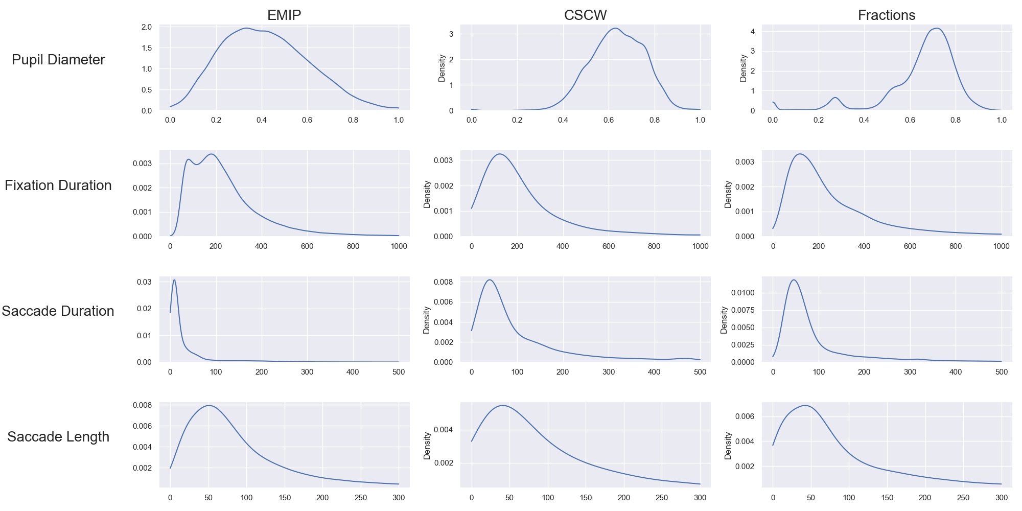
A.3. All Pipelines
| In Study Datasets | Out Of Study Dataset | Feature Group | PCA or LASSO | NRMSE | FGI |
|---|---|---|---|---|---|
cscw |
emip |
ARMA |
LASSO |
0.232 |
0.0076 |
cscw |
emip |
ARMA |
PCA |
0.24 |
0.0078 |
cscw |
emip |
All |
LASSO |
0.274 |
0.0079 |
cscw |
emip |
All |
PCA |
0.233 |
0.008 |
cscw |
emip |
Fixation Duration |
LASSO |
0.213 |
0.008 |
cscw |
emip |
Fixation Duration |
PCA |
0.24 |
0.008 |
cscw |
emip |
GARCH |
LASSO |
0.238 |
0.0081 |
cscw |
emip |
GARCH |
PCA |
0.235 |
0.008 |
cscw |
emip |
Gaze Characteristics |
LASSO |
0.215 |
0.0078 |
cscw |
emip |
Gaze Characteristics |
PCA |
0.22 |
0.0078 |
cscw |
emip |
HMM |
LASSO |
0.227 |
0.008 |
cscw |
emip |
HMM |
PCA |
0.197 |
0.0076 |
cscw |
emip |
Heatmaps |
LASSO |
0.206 |
0.0078 |
cscw |
emip |
Heatmaps |
PCA |
0.23 |
0.0077 |
cscw |
emip |
LHIPA |
LASSO |
0.262 |
0.0078 |
cscw |
emip |
LHIPA |
PCA |
0.207 |
0.0079 |
cscw |
emip |
Pupil Diameter |
LASSO |
0.186 |
0.0081 |
cscw |
emip |
Pupil Diameter |
PCA |
0.245 |
0.008 |
cscw |
emip |
Saccade Duration |
LASSO |
0.197 |
0.0079 |
cscw |
emip |
Saccade Duration |
PCA |
0.203 |
0.0081 |
cscw |
emip |
Saccade Length |
LASSO |
0.196 |
0.0081 |
cscw |
emip |
Saccade Length |
PCA |
0.249 |
0.008 |
cscw |
emip |
Spectral Histogram |
LASSO |
0.22 |
0.008 |
cscw |
emip |
Spectral Histogram |
PCA |
0.232 |
0.0081 |
cscw |
fractions |
ARMA |
LASSO |
0.202 |
0.0158 |
cscw |
fractions |
ARMA |
PCA |
0.183 |
0.0137 |
cscw |
fractions |
All |
LASSO |
0.205 |
0.0153 |
cscw |
fractions |
All |
PCA |
0.248 |
0.0179 |
cscw |
fractions |
Fixation Duration |
LASSO |
0.18 |
0.0139 |
cscw |
fractions |
Fixation Duration |
PCA |
0.2 |
0.0146 |
cscw |
fractions |
GARCH |
LASSO |
0.211 |
0.0144 |
cscw |
fractions |
GARCH |
PCA |
0.209 |
0.0135 |
cscw |
fractions |
Gaze Characteristics |
LASSO |
0.203 |
0.014 |
cscw |
fractions |
Gaze Characteristics |
PCA |
0.191 |
0.0141 |
cscw |
fractions |
HMM |
LASSO |
0.193 |
0.0149 |
cscw |
fractions |
HMM |
PCA |
0.238 |
0.0161 |
cscw |
fractions |
Heatmaps |
LASSO |
0.21 |
0.0147 |
cscw |
fractions |
Heatmaps |
PCA |
0.191 |
0.0137 |
cscw |
fractions |
LHIPA |
LASSO |
0.221 |
0.0152 |
cscw |
fractions |
LHIPA |
PCA |
0.249 |
0.0171 |
cscw |
fractions |
Pupil Diameter |
LASSO |
0.205 |
0.0155 |
cscw |
fractions |
Pupil Diameter |
PCA |
0.239 |
0.0179 |
cscw |
fractions |
Saccade Duration |
LASSO |
0.224 |
0.0156 |
cscw |
fractions |
Saccade Duration |
PCA |
0.217 |
0.0163 |
cscw |
fractions |
Saccade Length |
LASSO |
0.234 |
0.0144 |
cscw |
fractions |
Saccade Length |
PCA |
0.222 |
0.0151 |
cscw |
fractions |
Spectral Histogram |
LASSO |
0.184 |
0.0141 |
cscw |
fractions |
Spectral Histogram |
PCA |
0.22 |
0.0161 |
emip |
cscw |
ARMA |
LASSO |
0.323 |
0.0102 |
emip |
cscw |
ARMA |
PCA |
0.326 |
0.0107 |
emip |
cscw |
All |
LASSO |
0.354 |
0.0111 |
emip |
cscw |
All |
PCA |
0.304 |
0.0106 |
emip |
cscw |
Fixation Duration |
LASSO |
0.337 |
0.0102 |
emip |
cscw |
Fixation Duration |
PCA |
0.285 |
0.0101 |
emip |
cscw |
GARCH |
LASSO |
0.34 |
0.011 |
emip |
cscw |
GARCH |
PCA |
0.294 |
0.0105 |
emip |
cscw |
Gaze Characteristics |
LASSO |
0.327 |
0.0103 |
emip |
cscw |
Gaze Characteristics |
PCA |
0.304 |
0.0099 |
emip |
cscw |
HMM |
LASSO |
0.289 |
0.01 |
emip |
cscw |
HMM |
PCA |
0.301 |
0.0105 |
emip |
cscw |
Heatmaps |
LASSO |
0.353 |
0.0106 |
emip |
cscw |
Heatmaps |
PCA |
0.311 |
0.0101 |
emip |
cscw |
LHIPA |
LASSO |
0.307 |
0.0096 |
emip |
cscw |
LHIPA |
PCA |
0.279 |
0.0103 |
emip |
cscw |
Pupil Diameter |
LASSO |
0.249 |
0.0099 |
emip |
cscw |
Pupil Diameter |
PCA |
0.35 |
0.0104 |
emip |
cscw |
Saccade Duration |
LASSO |
0.335 |
0.01 |
emip |
cscw |
Saccade Duration |
PCA |
0.317 |
0.0102 |
emip |
cscw |
Saccade Length |
LASSO |
0.343 |
0.0106 |
emip |
cscw |
Saccade Length |
PCA |
0.325 |
0.0109 |
emip |
cscw |
Spectral Histogram |
LASSO |
0.319 |
0.0105 |
emip |
cscw |
Spectral Histogram |
PCA |
0.378 |
0.0114 |
emip |
fractions |
ARMA |
LASSO |
0.311 |
0.0164 |
emip |
fractions |
ARMA |
PCA |
0.345 |
0.0158 |
emip |
fractions |
All |
LASSO |
0.258 |
0.0125 |
emip |
fractions |
All |
PCA |
0.348 |
0.0159 |
emip |
fractions |
Fixation Duration |
LASSO |
0.336 |
0.0174 |
emip |
fractions |
Fixation Duration |
PCA |
0.348 |
0.0176 |
emip |
fractions |
GARCH |
LASSO |
0.32 |
0.0157 |
emip |
fractions |
GARCH |
PCA |
0.299 |
0.0138 |
emip |
fractions |
Gaze Characteristics |
LASSO |
0.335 |
0.017 |
emip |
fractions |
Gaze Characteristics |
PCA |
0.312 |
0.0178 |
emip |
fractions |
HMM |
LASSO |
0.287 |
0.017 |
emip |
fractions |
HMM |
PCA |
0.368 |
0.0191 |
emip |
fractions |
Heatmaps |
LASSO |
0.311 |
0.0165 |
emip |
fractions |
Heatmaps |
PCA |
0.293 |
0.0151 |
emip |
fractions |
LHIPA |
LASSO |
0.327 |
0.0127 |
emip |
fractions |
LHIPA |
PCA |
0.287 |
0.0104 |
emip |
fractions |
Pupil Diameter |
LASSO |
0.297 |
0.0124 |
emip |
fractions |
Pupil Diameter |
PCA |
0.372 |
0.018 |
emip |
fractions |
Saccade Duration |
LASSO |
0.336 |
0.0195 |
emip |
fractions |
Saccade Duration |
PCA |
0.307 |
0.0158 |
emip |
fractions |
Saccade Length |
LASSO |
0.355 |
0.0208 |
emip |
fractions |
Saccade Length |
PCA |
0.34 |
0.0165 |
emip |
fractions |
Spectral Histogram |
LASSO |
0.322 |
0.0172 |
emip |
fractions |
Spectral Histogram |
PCA |
0.361 |
0.0171 |
emip_cscw |
fractions |
ARMA |
LASSO |
0.29 |
0.01 |
emip_cscw |
fractions |
ARMA |
PCA |
0.259 |
0.0093 |
emip_cscw |
fractions |
All |
LASSO |
0.277 |
0.0117 |
emip_cscw |
fractions |
All |
PCA |
0.274 |
0.0093 |
emip_cscw |
fractions |
Fixation Duration |
LASSO |
0.258 |
0.0092 |
emip_cscw |
fractions |
Fixation Duration |
PCA |
0.3 |
0.0123 |
emip_cscw |
fractions |
GARCH |
LASSO |
0.246 |
0.009 |
emip_cscw |
fractions |
GARCH |
PCA |
0.247 |
0.0081 |
emip_cscw |
fractions |
Gaze Characteristics |
LASSO |
0.268 |
0.0102 |
emip_cscw |
fractions |
Gaze Characteristics |
PCA |
0.306 |
0.0114 |
emip_cscw |
fractions |
HMM |
LASSO |
0.277 |
0.0096 |
emip_cscw |
fractions |
HMM |
PCA |
0.303 |
0.0107 |
emip_cscw |
fractions |
Heatmaps |
LASSO |
0.284 |
0.0093 |
emip_cscw |
fractions |
Heatmaps |
PCA |
0.295 |
0.0092 |
emip_cscw |
fractions |
LHIPA |
LASSO |
0.279 |
0.0081 |
emip_cscw |
fractions |
LHIPA |
PCA |
0.304 |
0.0115 |
emip_cscw |
fractions |
Pupil Diameter |
LASSO |
0.288 |
0.0102 |
emip_cscw |
fractions |
Pupil Diameter |
PCA |
0.323 |
0.0112 |
emip_cscw |
fractions |
Saccade Duration |
LASSO |
0.267 |
0.0091 |
emip_cscw |
fractions |
Saccade Duration |
PCA |
0.301 |
0.0124 |
emip_cscw |
fractions |
Saccade Length |
LASSO |
0.287 |
0.0098 |
emip_cscw |
fractions |
Saccade Length |
PCA |
0.295 |
0.01 |
emip_cscw |
fractions |
Spectral Histogram |
LASSO |
0.261 |
0.0089 |
emip_cscw |
fractions |
Spectral Histogram |
PCA |
0.309 |
0.0131 |
fractions_emip |
cscw |
ARMA |
LASSO |
0.33 |
0.0099 |
fractions_emip |
cscw |
ARMA |
PCA |
0.278 |
0.0082 |
fractions_emip |
cscw |
All |
LASSO |
0.323 |
0.01 |
fractions_emip |
cscw |
All |
PCA |
0.323 |
0.0099 |
fractions_emip |
cscw |
Fixation Duration |
LASSO |
0.241 |
0.0084 |
fractions_emip |
cscw |
Fixation Duration |
PCA |
0.313 |
0.0102 |
fractions_emip |
cscw |
GARCH |
LASSO |
0.303 |
0.0093 |
fractions_emip |
cscw |
GARCH |
PCA |
0.288 |
0.0084 |
fractions_emip |
cscw |
Gaze Characteristics |
LASSO |
0.316 |
0.0094 |
fractions_emip |
cscw |
Gaze Characteristics |
PCA |
0.295 |
0.0091 |
fractions_emip |
cscw |
HMM |
LASSO |
0.304 |
0.0098 |
fractions_emip |
cscw |
HMM |
PCA |
0.311 |
0.0091 |
fractions_emip |
cscw |
Heatmaps |
LASSO |
0.377 |
0.011 |
fractions_emip |
cscw |
Heatmaps |
PCA |
0.325 |
0.01 |
fractions_emip |
cscw |
LHIPA |
LASSO |
0.33 |
0.0095 |
fractions_emip |
cscw |
LHIPA |
PCA |
0.283 |
0.0096 |
fractions_emip |
cscw |
Pupil Diameter |
LASSO |
0.295 |
0.0096 |
fractions_emip |
cscw |
Pupil Diameter |
PCA |
0.295 |
0.0097 |
fractions_emip |
cscw |
Saccade Duration |
LASSO |
0.33 |
0.0099 |
fractions_emip |
cscw |
Saccade Duration |
PCA |
0.324 |
0.0106 |
fractions_emip |
cscw |
Saccade Length |
LASSO |
0.303 |
0.0093 |
fractions_emip |
cscw |
Saccade Length |
PCA |
0.336 |
0.01 |
fractions_emip |
cscw |
Spectral Histogram |
LASSO |
0.278 |
0.0095 |
fractions_emip |
cscw |
Spectral Histogram |
PCA |
0.306 |
0.0103 |
fractions |
cscw |
ARMA |
LASSO |
0.247 |
0.0127 |
fractions |
cscw |
ARMA |
PCA |
0.302 |
0.0127 |
fractions |
cscw |
All |
LASSO |
0.266 |
0.013 |
fractions |
cscw |
All |
PCA |
0.213 |
0.0128 |
fractions |
cscw |
Fixation Duration |
LASSO |
0.283 |
0.0133 |
fractions |
cscw |
Fixation Duration |
PCA |
0.23 |
0.0128 |
fractions |
cscw |
GARCH |
LASSO |
0.252 |
0.0125 |
fractions |
cscw |
GARCH |
PCA |
0.316 |
0.0126 |
fractions |
cscw |
Gaze Characteristics |
LASSO |
0.174 |
0.0126 |
fractions |
cscw |
Gaze Characteristics |
PCA |
0.181 |
0.0125 |
fractions |
cscw |
HMM |
LASSO |
0.299 |
0.0129 |
fractions |
cscw |
HMM |
PCA |
0.314 |
0.0127 |
fractions |
cscw |
Heatmaps |
LASSO |
0.212 |
0.0126 |
fractions |
cscw |
Heatmaps |
PCA |
0.268 |
0.0124 |
fractions |
cscw |
LHIPA |
LASSO |
0.204 |
0.0125 |
fractions |
cscw |
LHIPA |
PCA |
0.324 |
0.0128 |
fractions |
cscw |
Pupil Diameter |
LASSO |
0.243 |
0.0129 |
fractions |
cscw |
Pupil Diameter |
PCA |
0.236 |
0.0128 |
fractions |
cscw |
Saccade Duration |
LASSO |
0.269 |
0.0134 |
fractions |
cscw |
Saccade Duration |
PCA |
0.322 |
0.0134 |
fractions |
cscw |
Saccade Length |
LASSO |
0.246 |
0.0125 |
fractions |
cscw |
Saccade Length |
PCA |
0.175 |
0.0122 |
fractions |
cscw |
Spectral Histogram |
LASSO |
0.216 |
0.0131 |
fractions |
cscw |
Spectral Histogram |
PCA |
0.318 |
0.0128 |
fractions |
emip |
ARMA |
LASSO |
0.331 |
0.0085 |
fractions |
emip |
ARMA |
PCA |
0.266 |
0.0087 |
fractions |
emip |
All |
LASSO |
0.246 |
0.0088 |
fractions |
emip |
All |
PCA |
0.286 |
0.0087 |
fractions |
emip |
Fixation Duration |
LASSO |
0.237 |
0.0088 |
fractions |
emip |
Fixation Duration |
PCA |
0.271 |
0.0085 |
fractions |
emip |
GARCH |
LASSO |
0.305 |
0.0087 |
fractions |
emip |
GARCH |
PCA |
0.277 |
0.0084 |
fractions |
emip |
Gaze Characteristics |
LASSO |
0.3 |
0.0088 |
fractions |
emip |
Gaze Characteristics |
PCA |
0.183 |
0.0089 |
fractions |
emip |
HMM |
LASSO |
0.339 |
0.0088 |
fractions |
emip |
HMM |
PCA |
0.294 |
0.0089 |
fractions |
emip |
Heatmaps |
LASSO |
0.24 |
0.0089 |
fractions |
emip |
Heatmaps |
PCA |
0.215 |
0.0086 |
fractions |
emip |
LHIPA |
LASSO |
0.293 |
0.0085 |
fractions |
emip |
LHIPA |
PCA |
0.278 |
0.0086 |
fractions |
emip |
Pupil Diameter |
LASSO |
0.341 |
0.0088 |
fractions |
emip |
Pupil Diameter |
PCA |
0.327 |
0.0087 |
fractions |
emip |
Saccade Duration |
LASSO |
0.295 |
0.0089 |
fractions |
emip |
Saccade Duration |
PCA |
0.166 |
0.009 |
fractions |
emip |
Saccade Length |
LASSO |
0.245 |
0.0087 |
fractions |
emip |
Saccade Length |
PCA |
0.265 |
0.0089 |
fractions |
emip |
Spectral Histogram |
LASSO |
0.221 |
0.0087 |
fractions |
emip |
Spectral Histogram |
PCA |
0.229 |
0.0089 |
fractions_cscw |
emip |
ARMA |
LASSO |
0.254 |
0.0076 |
fractions_cscw |
emip |
ARMA |
PCA |
0.285 |
0.0071 |
fractions_cscw |
emip |
All |
LASSO |
0.204 |
0.0078 |
fractions_cscw |
emip |
All |
PCA |
0.199 |
0.0074 |
fractions_cscw |
emip |
Fixation Duration |
LASSO |
0.243 |
0.0078 |
fractions_cscw |
emip |
Fixation Duration |
PCA |
0.256 |
0.0077 |
fractions_cscw |
emip |
GARCH |
LASSO |
0.227 |
0.007 |
fractions_cscw |
emip |
GARCH |
PCA |
0.274 |
0.0077 |
fractions_cscw |
emip |
Gaze Characteristics |
LASSO |
0.24 |
0.0075 |
fractions_cscw |
emip |
Gaze Characteristics |
PCA |
0.254 |
0.0072 |
fractions_cscw |
emip |
HMM |
LASSO |
0.226 |
0.0078 |
fractions_cscw |
emip |
HMM |
PCA |
0.245 |
0.0074 |
fractions_cscw |
emip |
Heatmaps |
LASSO |
0.214 |
0.0077 |
fractions_cscw |
emip |
Heatmaps |
PCA |
0.226 |
0.0077 |
fractions_cscw |
emip |
LHIPA |
LASSO |
0.251 |
0.0074 |
fractions_cscw |
emip |
LHIPA |
PCA |
0.246 |
0.0077 |
fractions_cscw |
emip |
Pupil Diameter |
LASSO |
0.259 |
0.0077 |
fractions_cscw |
emip |
Pupil Diameter |
PCA |
0.251 |
0.0077 |
fractions_cscw |
emip |
Saccade Duration |
LASSO |
0.221 |
0.0077 |
fractions_cscw |
emip |
Saccade Duration |
PCA |
0.26 |
0.0076 |
fractions_cscw |
emip |
Saccade Length |
LASSO |
0.229 |
0.0077 |
fractions_cscw |
emip |
Saccade Length |
PCA |
0.245 |
0.0076 |
fractions_cscw |
emip |
Spectral Histogram |
LASSO |
0.212 |
0.0074 |
fractions_cscw |
emip |
Spectral Histogram |
PCA |
0.26 |
0.0076 |